There is a new paper in press at the Journal of Climate that we were made aware of only a few days ago (July 14, 2010). It specifically addresses our (Spencer & Braswell, 2008, hereafter SB08) claim that previous satellite-based diagnoses of feedback have substantial low biases, due to natural variations in cloud cover of the Earth.

This is an important issue. If SB08 are correct, then the climate system could be substantially more resistant to forcings – such as increasing atmospheric CO2 concentrations — than the IPCC “consensus” claims it is. This would mean that manmade global warming could be much weaker than currently projected. This is an issue that Dick Lindzen (MIT) has been working on, too.

But if the new paper (MF10) is correct, then current satellite estimates of feedbacks – despite being noisy – still bracket the true feedbacks operating in the climate system…at least on the relatively short (~10 years) time scales of the satellite datasets. Forster and Gregory (2006) present some of these feedback estimates, based upon older ERBE satellite data.

As we will see, and as is usually the case, some of the MF10 criticism of SB08 is deserved, and some is not.

First, a Comment on Peer Review at the Journal of Climate

It is unfortunate that the authors and/or an editor at Journal of Climate decided that MF10 would be published without asking me or Danny Braswell to be reviewers.

Their paper is quite brief, and is obviously in the class of a “Comments on…” paper, yet it will appear as a full “Article”. But a “Comments on…” classification would then have required the Journal of Climate to give us a chance to review MF10 and to respond. So, it appears that one or more people wanted to avoid any inconvenient truths.

Thus, since it will be at least a year before a response study by us could be published – and J. Climate seems to be trying to avoid us – I must now respond here, to help avoid some of the endless questions I will have to endure once MF10 is in print.

On the positive side, though, MF10 have forced us to go back and reexamine the methodology and conclusions in SB08. As a result, we are now well on the way to new results which will better optimize the matching of satellite-observed climate variability to the simple climate model, including a range of feedback estimates consistent with the satellite data. It is now apparent to us that we did not do a good enough job of that in SB08.

I want to emphasize, though, that our most recent paper now in press at JGR (Spencer & Braswell, 2010: “On the Diagnosis of Radiative Feedback in the Presence of Unknown Radiative Forcing”, hereafter SB10), should be referenced by anyone interested in the latest published evidence supporting our claims. It does not have the main shortcomings I will address below.

But for those who want to get some idea of how we view the specific MF10 criticisms of SB08, I present the following. Keep in mind this is after only three days of analysis.

There are 2 Big Picture Questions Addressed by SB08 & MF10

There are two overarching scientific questions addressed by our SB08 paper, and MF10’s criticisms of it:

(1) Do significant low biases exist in current, satellite-based estimates of radiative feedbacks in the climate system (which could suggest high biases in inferred climate sensitivity)?

(2) Assuming that low biases do exist, did we (SB08) do an adequate job of demonstrating their probable origin, and how large those biases might be?

I will address question 1 first.

Big Picture Question #1: Does a Problem Even Exist in Diagnosing Feedbacks from Satellite Data?

MF10 conclude their paper with the claim that standard regression techniques can be applied to satellite data to get useful estimates of climate feedback, an opinion we strongly disagree with.

Fortunately, it is easy to demonstrate that a serious problem does exist. I will do this using MF10’s own method: analysis of output from coupled climate models. But rather than merely referencing a previous publication which does not even apply to the problem at hand, I will show actual evidence from 18 of the IPCC’s coupled climate models.

The following plot shows the final 10 years of data from the 20th Century run of the FGOALS model, output from which is archived at PCMDI (Meehl et al., 2007). The plot is global and 3-month averaged net radiative flux anomalies (reflected solar plus emitted infrared) versus the corresponding surface temperature anomalies produced by the model.

This represents the kind of data which are used to diagnose feedbacks from satellite data. The basic question we are trying to answer with such a plot is: “How much more radiant energy does the Earth lose in response to warming?” The answer to that question would help determine how strongly (or weakly) the climate system might respond to increasing CO2 levels.

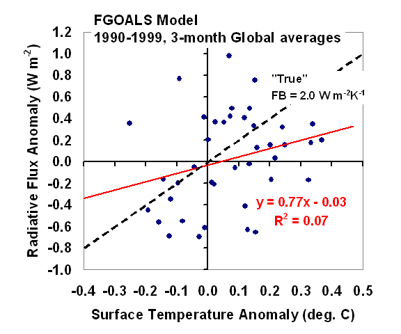
It is the slope of the red regression fit to the 3-month data points in the above figure that is the question: Is that slope an estimate of the net radiative feedback operating in the climate model, or not?

MF10 would presumably claim it is. We claim it is not, and furthermore that it will usually be biased low compared to the true feedback operating in the climate system. SB08 was our first attempt to demonstrate this with a simple climate model.

Well, the slope of 0.77 W m^-2 K^-1 in the above plot would correspond to a climate sensitivity in response to a doubling of atmospheric carbon dioxide (2XCO2) of (3.8/0.77=) 4.9 deg. C of global warming. [This assumes the widely accepted value near 3.8 W m^-2 K^-1 for the radiative energy imbalance of the Earth in response to 2XCO2].

But 4.9 deg. C of warming is more than DOUBLE the known sensitivity of this model, which is 2.0 to 2.2 deg. C (Forster & Taylor, J. Climate, 2006, hereafter FT06). This is clearly a large error in the diagnosed feedback.

As a statistician will quickly ask, though, does this error represent a bias common to most models, or is it just due to statistical noise?

To demonstrate this is no statistical outlier, the following plot shows regression-diagnosed versus “true” feedbacks diagnosed for 18 IPCC AR4 coupled climate models. We analyzed the output from the last 50 years of the 20th Century runs archived at PCMDI, computing average regression slopes in ten 5-year subsets of each model’s run, with 3-month average anomalies, then averaging those ten regression slopes for each model. Resulting climate sensitivities based upon those average regression slopes are shown separately for the 18 models in the next figure:

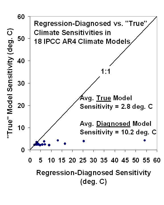
As can be seen, most models exhibit large biases – as much as 50 deg. C! — in feedback-inferred climate sensitivity, the result of low biases in the regression-diagnosed feedback parameters. Only 5 of the 18 IPCC AR4 models have errors in regression-inferred sensitivity less than 1 deg. C, and that is after beating down some noise with ten 5-year periods from each model! We can’t do that with only 10 years of satellite data.

Now, note that as long as such large inferred climate sensitivities (50+ deg.!?) can be claimed to be supported by the satellite data, the IPCC can continue to warn that catastrophic global warming is a real possibility.

The real reason why such biases exist, however, is addressed in greater depth in our new paper, (Spencer and Braswell, 2010). The low bias in diagnosed feedback (and thus high bias in climate sensitivity) is related to the extent to which time-varying radiative forcing, mostly due to clouds, contaminates the radiative feedback signal responding to temperature changes.

It is easy to get confused on the issue of using regression to estimate feedbacks because linear regression was ALSO used to get the “true” feedbacks in the previous figure. The difference is that, in order to do so, Forster and Taylor removed the large, transient CO2 radiative forcing imposed on the models in order to better isolate the radiative feedback signal. Over many decades of model run time, this radiative feedback signal then beats down the noise from non-feedback natural cloud variations.

Thus, diagnosing feedback accurately is fundamentally a signal-to-noise problem. Either any time-varying radiative forcing in the data must be relatively small to begin with, or it must be somehow estimated and then removed from the data.

It would be difficult to over-emphasize the importance of understanding the last paragraph.

So, Why Does the Murphy & Forster Example with the HadSM2 Model Give Accurate Feedbacks?

To support their case that there is no serious problem in diagnosing feedbacks from satellite data, MF10 use the example of Gregory et al. (2004 GRL, “A New Method for Diagnosing Radiative Forcing and Climate Sensitivity”). Gregory et al. analyzed the output of a climate model, HadSM3, and found that an accurate feedback could be diagnosed from the model output at just about any point during the model integration.

But the reason why Gregory et al. could do this, and why it has no consequence for the real world, is so obvious that I continue to be frustrated that so many climate experts still do not understand it.

The Gregory et al. HadSM3 model experiment used an instantaneous quadrupling (!) of the CO2 content of the model atmosphere. In such a hypothetical situation, there will be rapid warming, and thus a strong radiative feedback signal in response to that warming.

But this hypothetical situation has no analog in the real world. The only reason why one could accurately diagnose feedback in such a case is because the 4XCO2 radiative forcing is kept absolutely constant over time, and so the radiative feedback signal is not contaminated by it.

Again I emphasize, instantaneous and then constant radiative forcing has no analog in the real world. Experts using such unrealistic cases has led to much confusion regarding the diagnosis of feedbacks from satellite data. In nature, ever-evolving time-varying radiative forcings (what some call “unforced natural variability”) are almost always overpowering radiative feedback.

But does that mean that Spencer & Braswell (2008) did a convincing job of demonstrating how large the resulting errors in feedback diagnosis could be in response to such time-varying radiative forcing? Probably not.

Big Picture Question #2: Did Spencer & Braswell (2008) Do An Adequate Job of Demonstrating Why Feedback Biases Occur?

MF10 made two changes in our simple climate model which had large consequences: (1) they change the averaging time of the model output to be consistent with the relatively short satellite datasets we have to compare to, and (2) they increase the assumed depth of the tropical ocean mixed layer from 50 meters to 100 meters in the simple model.

The first change, we agree, is warranted, and it indeed results in less dramatic biases in feedbacks diagnosed from the simple model. We have independently checked this with the simple model by comparing our new results to those of MF10.

The second change, we believe, is not warranted, and it pushes the errors to even smaller values. If anything, we think we can show that even 50 meters is probably too deep a mixed layer for the tropical ocean (what we addressed) on these time scales.

Remember, we are exploring why feedbacks diagnosed from satellite-observed, year-to-year climate variability are biased low, and on those short time scales, the equivalent mixing depths are pretty shallow. As one extends the time to many decades, the depth of ocean responding to a persistent warming mechanism increases to 100’s of meters, consistent with MF10’s claim. But for diagnosing feedbacks from satellite data, the time scales of variability affecting the data are 1 to only a few years.

But we have also discovered a significant additional shortcoming in SB08 (and MF10) that has a huge impact on the answer to Question #2: In addition to just the monthly standard deviations of the satellite-measured radiative fluxes and sea surface temperatures, we should have included (at least) one more important satellite statistic: the level of decorrelation of the data.

Our SB10 paper actually does this (which is why it should be referenced for the latest evidence supporting our claims). After accounting for the decorrelation in the data (which exists in ALL of the IPCC models, see the first figure, above, for an example) the MF10 conclusion that the ratio of the noise to signal (N/S) in the satellite data is only around 15% can not be supported.

Unfortunately, SB08 did not adequately demonstrate this with the satellite data. SB10 does…but does not optimize the model parameters that best match the satellite data. That is now the focus of our new work on the subject.

Since this next step was not obvious to us until MF10 caused us to go back and reexamine the simple model and its assumptions, this shows the value of other researchers getting involved in this line of research. For that we are grateful.

Final Comments

While the above comments deal with the “big picture” issues and implications of SB08, and MF10’s criticism of it, there are also a couple of errors and misrepresentations in MF10 that should be addressed, things that could have been caught had we been allowed to review their manuscript.

1) MF10 claim to derive a “more correct” analytical expression for the error in feedback error than SB08 provided. If anything, it is ours that is more correct. Their expression (the derivation of which we admit is impressive) is only correct for an infinite time period, which is irrelevant to the issue at hand, and will have errors for finite time periods. In contrast, our expression is exactly correct for a finite time series of data, which is what we are concerned with in the real world.

2) MF10 remove “seasonal cycles” from the randomly forced model data time series. Why would this be necessary for a model that has only random daily forcing? Very strange.

Despite the shortcomings, MF10 do provide some valuable insight, and some of what they present is indeed useful for advancing our understanding of what causes variations in the radiative energy budget of the Earth.

References
Forster, P. M., and J. M. Gregory (2006), The climate sensitivity and its components diagnosed from Earth Radiation Budget data, J. Climate, 19, 39-52.

Forster, P.M., and K.E. Taylor (2006), Climate forcings and climate sensitivities diagnosed from coupled climate model integrations, J. Climate, 19, 6181-6194.

Gregory, J.M., W. J. Ingram, M.A. Palmer, G.S. Jones, P.A. Stott, R.B. Thorpe, J.A. Lowe, T.C Johns, and K.D. Williams (2004), A new method for diagnosing radiative forcing and climate sensitivity, Geophys. Res. Lett., 31, L03205, doi:10.1029/2003GL018747.

Meehl, G. A., C. Covey, T. Delworth, M. Latif, B. McAvaney, J. F. B. Mitchell, R. J. Stouffer, and K. E. Taylor (2007), The WCRP CMIP3 multi-model dataset: A new era in climate change research, Bull. Am. Meteorol. Soc., 88, 1383-1394.

Murphy, D.M., and P. M. Forster (2010), On the Accuracy of Deriving Climate Feedback Parameters from Correlations Between Surface Temperature and Outgoing Radiation. J. Climate, in press. [PDF currently available to AMS members].

Spencer, R.W., and W.D. Braswell (2008), Potential biases in cloud feedback diagnosis: A simple model demonstration, J. Climate, 21, 5624-5628. PDF.

Spencer, R. W., and W. D. Braswell (2010), On the Diagnosis of Radiative Feedback in the Presence of Unknown Radiative Forcing, J. Geophys. Res., doi:10.1029/2009JD013371, in press. [PDF currently available to AGU members] (accepted 12 April 2010)