After yesterday’s post, I decided to run the simple forcing-feedback model we developed to mimic the Aqua satellite observations of global oceanic temperature and radiative flux variations.

I’ve also perused the comments people have made there, and will try to clarify what I’ve done and why it’s important.

First of all, my (and even the IPCC’s) emphasis on changes in the global radiative budget cannot be overemphasized when we are trying to figure out whether “global warming” is mostly manmade or natural, and how the climate system responds to forcing.

Changes in the global-average radiative budget are about the only way for the Earth to warm or cool on time scales of years or longer (unless there is some sort of change in geothermal heat flux…we won’t even go there.)

What we want to know, ultimately, is how much warming will result from the radiative imbalance caused by adding CO2 to the atmosphere. It is natural to try to answer that question by examining how Mother Nature handles things when there are natural, year-to-year warmings and coolings. I believe that the NASA satellite assets we have in orbit right now are going to go a long way toward providing that answer.

The answer depends upon how clouds, evaporation, water vapor, etc., change IN RESPONSE TO a temperature change, thus further altering the radiative balance and final temperature response. This is called feedback, and it is traditionally referenced to a surface temperature change.

The GOOD news is that we have pretty accurate satellite measurements of the rather small, year-to-year changes in global radiative fluxes over the last 10 years, as well as of the temperature changes that accompanied them.

The BAD news is that, even if those measurements were perfect, determining feedback (temperature causing radiative changes) is confounded by natural forcings (radiative changes causing temperature changes).

This interplay between natural variations in global-average temperature and radiative flux are always occurring, intermingled together, and the goal is to somehow disentangle them to get at the feedback part.

Keep in mind that “feedback” in the climate system is more of a conceptual construct. It isn’t something we can measure directly with an instrument, like temperature. But the feedback concept is useful because we are pretty sure that elements of the climate system (e.g. clouds) WILL change in response to any radiative imbalance imposed upon the system, and those changes will either AMPLIFY or REDUCE the temperature changes resulting from the initial imbalance. (While it might not be exactly the same kind of feedback electrical engineers deal with, there is currently no better term to describe the process…a process which we know must be occurring, and must be understood in order to better predict human-caused global warming.)

More than any other factor, feedbacks will determine whether anthropogenic global warming is something we need to worry about.

An Example from the Kitchen
While this might all seem rather cryptic, ALL of these processes have direct analogs to a pot of water warming on the stove. You can turn the heat up on the stove (forcing), and the water will warm. But if you also remove the lid in proportion to the stove being turned up (negative feedback), you can reduce the warming. It’s all based upon energy conservation concepts, which ordinary people are exposed to every day.

The IPCC believes Mother Nature covers up the pot even more as the stove is turned up, causing even more warming in response to a “forcing”.

I think they are wrong.

NASA Aqua Satellite Observations of the Global Oceans
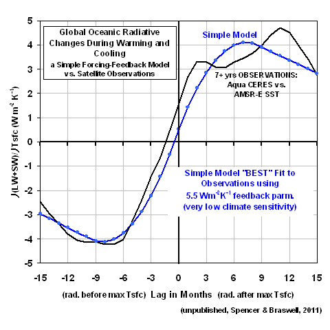
Similar to what I plotted yesterday, the following plot shows time-lagged regression coefficients between time series of global oceanic radiative flux (from the CERES instrument on Aqua), and sea surface temperature (from AMSR-E on Aqua). Yesterday’s plot also showed the results when I used the Hadley Center’s SST measurements (the dashed line in that graph), and the results were almost identical. But since I’m the U.S. Science Team Leader for AMSR-E, I’ll use it instead. 🙂

The way these regression coefficients can be interpreted is that they quantify the rate at which radiative energy is GAINED by the global ocean during periods when SST is rising, and the rate at which radiative energy is LOST when SST is falling. Conceptually, the vertical line at zero months time lag can be thought of as corresponding to the time of peak SST.

The Simple Model “Best” Match to the Satellite Data
I’ve run our simple forcing-feedback model (originally suggested to us by Isaac Held at Princeton) to try to match the satellite observations. I force the model with quasi-random time variations in the global radiative energy budget — representing, say, natural, quasi-chaotic variations in cloud cover — and then see how the model temperatures respond. The model has been available here for many months now, if you want to play with it.

The model’s response to these radiative forcings depends upon how I set the model’s: (1) ocean mixing depth, which will determine how much the temperature will change for a given energy imbalance imposed upon the model, and (2) feedback parameter, which is what we ultimately want to determine from the satellite data.

I found that a 70 meter deep layer provided about the right RATIO between the satellite-observed monthly radiative variations (0.8 Watts per sq. meter standard deviation) and SST variations (0.08 deg. C standard deviation). At the same time, I had to adjust the magnitude of the radiative forcing to get about the right ABSOLUTE MAGNITUDES for those standard deviation statistics, too.

The “best fit” I got after about an hour of fiddling around with the inputs is represented by the blue curve in the above chart. Importantly, the assumed feedback parameter (5.5) is solidly in “negative feedback” territory. IF this was the true feedback operating in the real climate system on the long time scales of ‘global warming’, it would mean that our worries over anthropogenic global warming have been, for all practical purposes, a false alarm.

The Simple Model Run With the IPCC’s Average Feedback

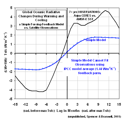
At this point, a natural question is, How does the simple model behave if I run it with a feedback typical of the IPCC climate models? The average net feedback parameter across the IPCC models is about 1.4 Watts per sq. meter per degree, and the following plot shows the simple model’s response to that feedback value compared to the satellite observations.

A comparison between the 2 charts above would seems to indicate that the satellite data are more consistent with negative feedback (which, if you are wondering, is a net feedback parameter greater than 3.2 W m-2 K-1) than they are with positive feedback. But it could be that feedbacks diagnosed from the IPCC models only over the global oceans will be necessary to provide a more apples-to-apples comparison on this point.

Important Caveat
While it would be tempting to think that the IPCC models are potentially invalidated by this comparison, Dessler (2010) has correctly pointed out that the short-term feedback behavior of the IPCC models appear to have little or no relationship to their long-term climate sensitivity.

In other words, even if short-term feedbacks in the real climate system are strongly negative, this doesn’t prove the long-term global warming in the models is wrong.

In fact, NO ONE HAS YET FOUND A WAY WITH OBSERVATIONAL DATA TO TEST CLIMATE MODEL SENSITIVITY. This means we have no idea which of the climate models projections are more likely to come true.

This dirty little secret of the climate modeling community is seldom mentioned outside the community. Don’t tell anyone I told you.

This is why climate researchers talk about probable ranges of climate sensitivity. Whatever that means!…there is no statistical probability involved with one-of-a-kind events like global warming!

There is HUGE uncertainty on this issue. And I will continue to contend that this uncertainty is a DIRECT RESULT of researchers not distinguishing between cause and effect when analyzing data.

Toward Improved Climate Sensitivity Estimates
As I mentioned yesterday, Dessler (2010) only addressed ZERO-time lag relationships, as did all previous investigators doing similar kinds of work. In contrast, the plots I am presenting here (and in yesterday’s post) show how these regression coefficients vary considerably with time lag. In fact, at zero time lag, the relationships become virtually meaningless. Cause and effect are hopelessly intertwined.

But we CAN measure radiative changes BEFORE a temperature peak is reached, and in the months FOLLOWING the peak. Using such additional “degrees of freedom” in data analysis will be critical if we are to ever determine climate sensitivity from observational data. I know that Dick Lindzen is also advocating the very same point. If you are a lay person who understands this, can i get an “amen”? Because, so far, other climate researchers are keeping their mouths shut.

It is imperative that the time lags (at a minimum) be taken into account in such studies. Our previous paper (Spencer & Braswell, 2010) used phase space plots as a way of illustrating time lag behavior, but it could be that plots like I have presented here would be more readily understood by other scientists.

Unfortunately, the longer the climate community establishment keeps its head in the sand on this issue , the more foolish they will look in the long run.