INTRODUCTION
My last few posts have described a new method for quantifying the average Urban Heat Island (UHI) warming effect as a function of population density, using thousands of pairs of temperature measuring stations within 150 km of each other. The results supported previous work which had shown that UHI warming increases logarithmically with population, with the greatest rate of warming occurring at the lowest population densities as population density increases.

But how does this help us determine whether global warming trends have been spuriously inflated by such effects remaining in the leading surface temperature datasets, like those produced by Phil Jones (CRU) and Jim Hansen (NASA/GISS)?

While my quantifying the UHI effect is an interesting exercise, the existence of such an effect spatially (with distance between stations) does not necessarily prove that there has been a spurious warming in the thermometer measurements at those stations over time. The reason why it doesn’t is that, to the extent that the population density of each thermometer site does not change over time, then various levels of UHI contamination at different thermometer sites would probably have little influence on long-term temperature trends. Urbanized locations would indeed be warmer on average, but “global warming” would affect them in about the same way as the more rural locations.

This hypothetical situation seems unlikely, though, since population does indeed increase over time. If we had sufficient truly-rural stations to rely on, we could just throw all the other UHI-contaminated data away. Unfortunately, there are very few long-term records from thermometers that have not experienced some sort of change in their exposure…usually the addition of manmade structures and surfaces that lead to spurious warming.

Thus, we are forced to use data from sites with at least some level of UHI contamination. So the question becomes, how does one adjust for such effects?

As the provider of the officially-blessed GHCN temperature dataset that both Hansen and Jones depend upon, NOAA has chosen a rather painstaking approach where the long-term temperature records from individual thermometer sites have undergone homogeneity “corrections” to their data, mainly based upon (presumably spurious) abrupt temperature changes over time. The coming and going of some stations over the years further complicates the construction of temperature records back 100 years or more.

All of these problems (among others) have led to a hodgepodge of complex adjustments.

A SIMPLER TECHNIQUE TO LOOK FOR SPURIOUS WARMING

I like simplicity of analysis — whenever possible, anyway. Complexity in data analysis should only be added when it is required to elucidate something that is not obvious from a simpler analysis. And it turns out that a simple analysis of publicly available raw (not adjusted) temperature data from NOAA/NESDIS NOAA/NCDC, combined with high-resolution population density data for those temperature monitoring sites, shows clear evidence of UHI warming contaminating the GHCN data for the United States.

I will restrict the analysis to 1973 and later since (1) this is the primary period of warming allegedly due to anthropogenic greenhouse gas emissions; (2) the period having the largest number of monitoring sites has been since 1973; and (3) a relatively short 37-year record maximizes the number of continuously operating stations, avoiding the need to handle transitions as older stations stop operating and newer ones are added.

Similar to my previous posts, for each U.S. station I average together four temperature measurements per day (00, 06, 12, and 18 UTC) to get a daily average temperature (GHCN uses daily max/min data). There must be at least 20 days of such data for a monthly average to be computed. I then include only those stations having at least 90% complete monthly data from 1973 through 2009. Annual cycles in temperature and anomalies are computed from each station separately.

I then compute multi-station average anomalies in 5×5 deg. latitude/longitude boxes, and then compare the temperature trends for the represented regions to those in the CRUTem3 (Phil Jones’) dataset for the same regions. But to determine whether the CRUTem3 dataset has any spurious trends, I further divide my averages into 4 population density classes: 0 to 25; 25 to 100; 100 to 400; and greater than 400 persons per sq. km. The population density data is at a nominal 1 km resolution, available for 1990 and 2000…I use the 2000 data.

All of these restrictions then result in thirteen 24 to 26 5-deg grid boxes over the U.S. having all population classes represented over the 37-year period of record. In comparison, the entire U.S. covers about 31 40 grid boxes in the CRUTem3 dataset. While the following results are therefore for a regional subset (at least 60%) of the U.S., we will see that the CRUTem3 temperature variations for the entire U.S. do not change substantially when all 31 40 grids are included in the CRUTem3 averaging.

EVIDENCE OF A LARGE SPURIOUS WARMING TREND IN THE U.S. GHCN DATA

The following chart shows yearly area-averaged temperature anomalies from 1973 through 2009 for the 13 24 to 26 5-deg. grid squares over the U.S. having all four population classes represented (as well as a CRUTem3 average temperature measurement). All anomalies have been recomputed relative to the 30-year period, 1973-2002.

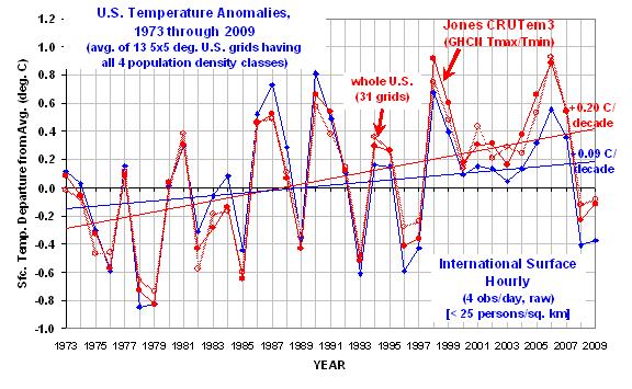
The heavy red line is from the CRUTem3 dataset, and so might be considered one of the “official” estimates. The heavy blue curve is the lowest population class. (The other 3 population classes clutter the figure too much to show, but we will soon see those results in a more useful form.)

Significantly, the warming trend in the lowest population class is only 47% of the CRUTem3 trend, a factor of two difference.

Also interesting is that in the CRUTem3 data, 1998 and 2006 would be the two warmest years during this period of record. But in the lowest population class data, the two warmest years are 1987 and 1990. When the CRUTem3 data for the whole U.S. are analyzed (the lighter red line) the two warmest years are swapped, 2006 is 1st and then 1998 2nd.

From looking at the warmest years in the CRUTem3 data, one gets the impression that each new high-temperature year supersedes the previous one in intensity. But the low-population stations show just the opposite: the intensity of the warmest years is actually decreasing over time.

To get a better idea of how the calculated warming trend depends upon population density for all 4 classes, the following graph shows – just like the spatial UHI effect on temperatures I have previously reported on – that the warming trend goes down nonlinearly as population density of the stations decrease. In fact, extrapolation of these results to zero population density might produce little warming at all!

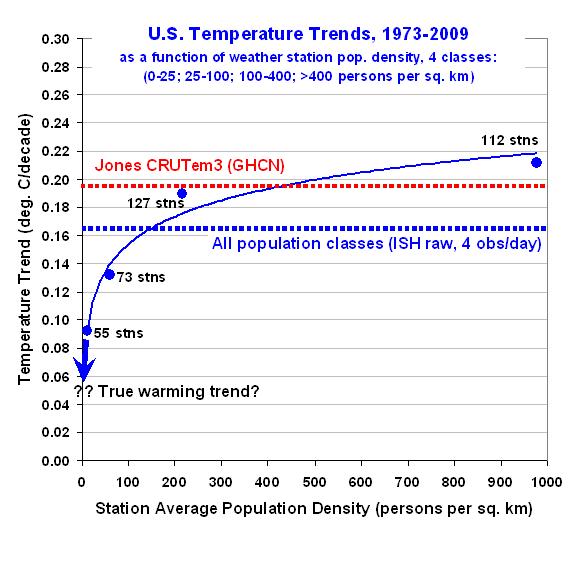
This is a very significant result. It suggests the possibility that there has been essentially no warming in the U.S. since the 1970s.

Also, note that the highest population class actually exhibits slightly more warming than that seen in the CRUTem3 dataset. This provides additional confidence that the effects demonstrated here are real.

Finally, the next graph shows the difference between the lowest population density class results seen in the first graph above. This provides a better idea of which years contribute to the large difference in warming trends.

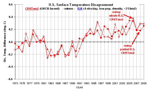
Taken together, I believe these results provide powerful and direct evidence that the GHCN data still has a substantial spurious warming component, at least for the period (since 1973) and region (U.S.) addressed here.

There is a clear need for new, independent analyses of the global temperature data…the raw data, that is. As I have mentioned before, we need independent groups doing new and independent global temperature analyses — not international committees of Nobel laureates passing down opinions on tablets of stone.

But, as always, the analysis presented above is meant more for stimulating thought and discussion, and does not equal a peer-reviewed paper. Caveat emptor.