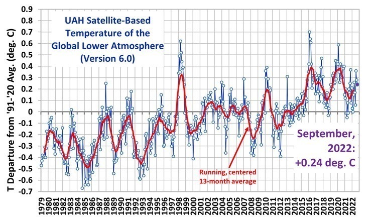
Archive for the ‘Blog Article’ Category

Could Recent U.S. Warming Trends be Largely Spurious?

Friday, January 29th, 2021

Several lines of evidence suggest observed warming trends are not nearly as large as what you have been told.

It’s been almost eight years since I posted results on my analysis of the global Integrated Surface Database (ISD) temperature data. Despite finding evidence that urbanization effects on temperature measurements have not been removed from official land temperature datasets, I still refer people to the official products (e.g. from NOAA GHCN, HadCRUT, etc.). This is because I never published any results from my analysis.

But I’ve started thinking again about the question, Just how much warming has there been in recent decades (say, the last 50 years)? The climate models suggest that this should have been the period of most rapid warming, due to ever-increasing atmospheric CO2 combined with a reduction in aerosol pollution. Since those models are the basis for proposed changes in energy policy, it is important that the observations to which they are compared be trustworthy.

A Review of the Diagnosed Urban Heat Island Effect

The official datasets of land surface temperature are (we are told) already adjusted for Urban Heat Island (UHI) effects. But as far as I know, it has never been demonstrated that the spurious warming from urban effects have been removed. Making temperature trends be the same independent of urbanization does NOT mean urban warming effects have been removed. It could be that spurious warming has simply been spread around to the non-affected stations.

Back in 2010 I quantified the Urban Heat Island (UHI) effect, based upon the difference in absolute temperatures between closely-spaced neighboring stations having different population densities (PD). The ISD temperature data are not max/min (as in GHCN), but data taken hourly, with the longest-record stations reporting at just the 6-hourly synoptic times (00, 06, 12, 18 UTC). Because there were many more stations added to the global dataset in 1973, all of my analyses started then.

By using many station pairs from low to high population densities, I constructed the cumulative UHI effect as a function of population density. Here are the results from global data in the year 2000:

Fig. 1. Diagnosed average Urban Heat Island warming in 2000 from over 11,000 closely spaced station pairs having different population densities.

As can be seen, the largest warming effect with a change in population density occurs at the lowest population densities (not a new finding), with the most total warming at the highest population densities.

The Effect of Population Density on U.S. Station Temperature Trends

In 2012 I experimented with methods to removed the observed UHI effect in the raw ISD 6-hourly data using population density as a proxy. As you can see in the second of the two graphs below, the highest population density stations had ~0.25 C/decade warming trend, with a reduced warming trend as population density was reduced:

Fig. 2. U.S. surface temperature trends as a function of local population density at the station locations: top (raw), bottom (averages into 4 groups).

Significantly, extrapolating to zero population density would give essentially no warming in the United States during 1973-2011. As we shall see (below) official temperature datasets say this period had a substantial warming trend, consistent with the warming in the highest population density locations.

How can one explain this result other than, at least for the period 1973-2011, (1) spurious warming occurred at the higher population density stations, and (2) the evidence supports essentially no warming if there were no people (zero population density) to modify the microclimate around thermometer sites?

I am not claiming there has been no global warming (whatever the cause). I am claiming that there is evidence of spurious warming in thermometer data which must be removed.

Next, we will examine how well that effect has been removed.

How Does this Compare to the ‘Official’ Temperature Trends?

Since I performed these analyses almost 10 years ago, the ‘official’ temperature datasets have been adjusted several times. For the same period I analyzed 8-10 years years ago, look at how some of these datasets have increased the temperature trends (I used only CRUTem3 back then):

Fig. 3. U.S. surface temperature trend from different datasets.

The CRUTem3 data produce a trend reasonably close to the raw, unadjusted 6-hourly ISD-based data (the correlation of the two datasets’ monthly anomaly time series was 0.994). Note that the latest USHCN data in the above graph has the most warming, at +0.26 C/decade.

Note that this is about the same as the trend I get with the stations having the highest (rather than lowest) population density. Anthony Watts reported qualitatively similar results using different data back in 2015.

How in the world can the warming result from NOAA be reconciled with the (possible zero warming) results in Fig. 2? NOAA uses a complex homogenization procedure to make its adjustments, but it seems to me the the results in Fig. 2 suggest that their procedures might be causing spurious warming trends in the data. I am not the first to point this out; others have made the same claims over the years. I am simply showing additional quantitative evidence.

I don’t see how it can be a change in instrumentation, since both rural and urban stations changed over the decades from liquid-in-glass thermometers in Stevenson screens, to digital thermistors in small hygrothermometer enclosures, to the new automated ASOS measurement systems.

Conclusion

It seems to me that there remains considerable uncertainty in just how much the U.S. has warmed in recent decades, even among the established, official, ‘homogenized’ datasets. This has a direct impact on the “validation” of climate models relied upon by the new Biden Administration for establishing energy policy.

I would not be surprised if such problems exist in global land temperature datasets in addition to the U.S.

I’m not claiming I know how much it has (or hasn’t) warmed. Instead, I’m saying I am still very suspicious of existing official land temperature datasets.

Biden to End Fossil Fuel Subsidies: Like the Paris Agreement, it Will Make No Difference

Wednesday, January 27th, 2021

Joe Biden’s administration has made climate change one of its top priorities. Photographer: Doug Mills/The New York Times/Bloomberg

In what appears to be a never-ending string of ineffective efforts to force the public to use expensive, unreliable, intermittent, and not-widely-deployable renewable energy, the Biden Administration is issuing an executive order that (among other things) directs federal agencies to end fossil fuel subsidies.

Personally, I would not mind if all federal subsidies were ended, since all that subsidies do is put the government, rather than the consumer, in charge of what you spend your money on.

But federal subsidies on fossil fuels represent less that 3% of the revenues of the fossil fuel industry. This action will have essentially no impact on an economy that still runs on fossil fuels. That 3% will be voluntarily paid by the consumer, just directly rather than through subsidies.

In contrast, renewables currently enjoy 25 times the level of subsides per unit of energy produced as do fossil fuels, and the market penetration of EVs is still only 1.2%. One can see that massive government meddling in the energy market is the only way that people will — at least for the foreseeable future — “choose” renewables over fossil fuels.

So, while environmentalists might applaud Biden’s decision, the effect on the energy markets will be barely measurable, if at all.

You see, when it comes to global warming, modern environmentalism depends upon feelings over facts. Even if all CO2 emissions in the U.S. were to end, the impact on global temperatures by 2100 would be small. This is because the U.S. now produces less than 15% of the global total greenhouse gas emissions. The same is true if all countries abide by their commitments under the Paris Climate Agreement, which makes Biden’s rejoining that Agreement rather pointless. The effect of Paris is calculated to be a 0.2 deg. C reduction in warming by 2100, which is too small to measure over the next 80 years with temperature monitoring technologies currently in place.

Even the godfather of modern global warming alarmism, NASA’s James Hansen says the Paris Agreement is ineffective and a “fraud”, and that only massive taxation of (i.e. punishment for) using fossil fuels will make much difference.

To show just how much CO2 emissions will have to decrease to affect the atmospheric CO2 concentration, just look at what happened (or didn’t happen) last year. The U.S. Energy Information Agency (EIA) estimates that the economic downturn in 2020 produced only an 11% reduction in fossil fuel use. The resulting change in atmospheric CO2 concentration was unmeasurable:

The 11% reduction in global CO2 emissions in 2020 had no measurable impact on atmospheric CO2 concentrations at Mauna Loa, Hawaii.

Furthermore, while we nibble around the edges of the “carbon pollution” problem, China’s CO2 emissions continue to grow.

The U.S. has led the way in reducing CO2 emissions, mainly through a market-driven switch from coal to natural gas in recent years, China’s emissions continue to grow.

And while the “social cost of carbon” continues to be advanced as the justification for reducing CO2 emissions, no one wants to talk about the social benefits. For example, Nature loves the stuff. It is estimated that global agricultural productivity has increased by $3.5 Trillion from the extra CO2 in the atmosphere. It is well known that excessive cold kills far more people than excessive heat. There is no evidence that recent, modest global warming has caused a global-average increase in severe weather.

The claims by China that they will become “carbon neutral” by 2060 is just political posturing. One thing I have learned about China in recent decades is that their political culture is to say anything necessary to nominally appease other countries, and then do just the opposite if it suits their national interests. With over four times the population of the U.S., one can see why they would not want the U.S. (or any other county) dictating their behavior, especially as they continue to lift millions out of poverty.

Not unless the Biden Administration pushes for a massive increase in the taxation of fossil fuels, and then embraces either nuclear plant construction or widespread wind and solar projects to service a huge fleet of electric vehicles (currently at 1.2% of U.S. market penetration) will there be any substantial move away from fossil fuels.

Anything less will only falsely assuage fears rather than address facts.

Canada is Warming at Only 1/2 the Rate of Climate Model Simulations

Thursday, January 21st, 2021

As part of my Jan. 19 presentation for Friends of Science about there being no climate emergency, I also examined surface temperature in Canada to see how much warming there has been compared to climate models.

Canada has huge year-to-year variability in temperatures due to its strong continental climate. So, to examine how observed surface temperature trends compare to climate model simulations, you need many of those simulations, each of which exhibits its own large variability.

I examined the most recent 30-year period (1991-2020), using a total of 108 CMIP5 simulations from approximately 20 different climate models, and computed land-surface trends over the latitude bounds of 51N to 70N, and longitude bounds 60W to 130W, which approximately covers Canada. For observations, I used the same lat/lon bounds and the CRUTem5 dataset, which is heavily relied upon by the UN IPCC and world governments. All data were downloaded from the KNMI Climate Explorer.

First let’s examine the annual average temperature departures from the 1981-2010 average, for the average of the 108 model simulations compared to the observations. We see that Canada has been warming at only 50% the rate of the average of the CMIP5 models; the linear trends are +0.23 C/decade and +0.49 C/decade, respectively. Note that in 7 of the last 8 years, the observations have been below the average of the models.

Fig. 1. Yearly temperature departures 1991-2020 from the 1981-2010 mean in Canada in observations (blue) versus the average of 108 CMIP5 climate model simulations (red). The +/-1 standard deviation bars indicate the variability among the 108 individual model simulations.

Next, I show the individual models’ trends compared to the observed trends, with a histogram of the ranked values from the least warming to the most warming, 1991-2020.

Fig. 2. Ranked Canada surface temperature trends (1991-2020) for the 108 model simulations and the observations.

Note that the 93.5% of the model simulations have warmer temperature trends than the observations exhibit.

These results from Canada are generally consistent with the results I have found in the Midwest U.S. in the summertime, where the CMIP5 models warm, on average, 4 times faster than the observations (since 1970), and 6 times faster in a limited number of the newer CMIP6 model simulations.

Implications

The Paris Climate Accords, among other national and international efforts to reduce greenhouse gas emissions, assume warming estimates which are approximately the average of the various climate models. Thus, these results impact directly on those proposed energy policy decisions.

As you might be aware, proponents of those climate models often emphasize the general agreement between the models and observations over a long period of time, say since 1900.

But this is misleading.

We would expect little anthropogenic global warming signal to emerge from the noise of natural climate variability until (approximately) the 1980s. This is for 2 reasons: There was little CO2 emitted up through the 1970s, and even as the emissions rose after the 1940s the cooling effect of anthropogenic SO2 emissions was canceling out much of that warming. This is widely agreed to by climate modelers as well.

Thus, to really get a good signal of global warming — in both observations and models — we should be examining temperature trends since approximately the 1980s. That is, only in the decades since the 1980s should we be seeing a robust signal of anthropogenic warming against the background of natural variability, and without the confusion (and uncertainty) in large SO2 emissions in the mid-20th century.

And as each year passes now, the warming signal should grow slightly stronger.

I continue to contend that climate models are now producing at least twice as much warming as they should, probably due to an equilibrium climate sensitivity which is about 2X too high in the climate models. Given that the average CMIP6 climate sensitivity is even larger than in CMIP5 — approaching 4 deg. C — it will be interesting to see if the divergence between models and observations (which began around the turn of the century) will continue into the future.


This Tuesday, Jan. 19: My Friends of Science Society Livestream Talk: ‘Why There Is No Climate Emergency’

Friday, January 15th, 2021

On Tuesday evening, January 19, at 8 p.m. CST there will be a 30 minute livestream presentation where I cover the most important reasons why there is no climate emergency. I just reviewed the video and I am very satisfied with it.

In only 1/2 hour I cover what I consider to be the most important science issues, the disinformation campaign that spreads climate hysteria, some of the harm that will be caused by forcing expensive and unreliable renewable energy upon humanity, and the benefits of more CO2 in the atmosphere.

You can go to the FoS website for more information. The tickets are $15, and I will be doing a live Q&A after the event.

No, Roy Spencer is not a climate “denier”

Wednesday, January 13th, 2021

Yesterday, the New York Times and other media outlets repeated the falsehood that I am a climate “denier”.

I usually ignore such potentially libelous statements, otherwise I’d be defending myself every week.

So, to set the record straight, here’s what I believe… I’ll let you decide whether I’m a climate “denier”.

  1. I believe the climate system has warmed (we produce one of the global datasets that shows just that, which is widely used in the climate community), and that CO2 emissions from fossil fuel burning contributes to that warming. I’ve said this for many years.
  2. I believe future warming from a doubling of atmospheric CO2 would be somewhere in the range of 1.5 to 2 deg. C, which is actually within the range of expected warming the UN Intergovernmental Panel on Climate Change (IPCC) has advanced for 30 years now. (It could be less than this, but we simply don’t know).

As people who frequent this blog well know, I have held these views for many years. I routinely take other skeptics to task for believing such things as “there is no greenhouse effect”, or “it’s impossible for a cold atmosphere to make the Earth’s surface even warmer”.

So, Why Is Roy Spencer Called a Climate Denier?

In the case of global warming, alarmists apparently insist that you must believe that global warming is a “crisis” or an “emergency”, or else you will be thrown under the bus.

They claim we must embrace expensive (and ineffective) sources of alternative energy. But, like Bjorn Lomborg (who actually believes the alarmist predictions of future warming) and many others, I believe it will be much worse for humanity if we abandon fossil fuels before alternative technologies are abundant, affordable, and practical.

Human flourishing requires access to affordable energy, which is required for almost all human activities. It is immoral to deny fossil-fueled electricity to the world’s poor, and its replacement in even the richest countries still destroys prosperity, especially for the poor.

For believing these things, I am declared evil, apparently on par with a Holocaust denier (thus the rhetoric).

Here’s some of that rhetoric from the Daily Kos yesterday, which covered the firing of White House skeptical scientists Dr. David Legates and Dr. Ryan Maue (emphasis added):

“The bundle of boring and basic denial myths compiled to appease the deadly denial of the Trump administration was published first, it appears at least, by U-Alabama Huntsville’s Dr. Roy Spencer, who contributed a chapter. His post about the flyers was then bounced around the deniersphere, where the same audiences who gobble up unhinged conspiracies about voter fraud or satan-worshipping Democrats can eagerly read the climate denial versions of those violent fantasies.”

This is apparently what happens when you take frustrated creative writers and give them jobs as journalists.

Given recent political events it appears there is now a renewed efforts to have dissenting voices silenced through “cancel culture”, removal of websites, public ridicule, censorship, etc.

Unity in our country will, apparently, be achieved, because once dissenting voices are silenced, “unity” is all that is left.

At the White House, the Purge of Skeptics Has Started

Tuesday, January 12th, 2021

Dr. David Legates has been Fired by White House OSTP Director and Trump Science Advisor, Kelvin Droegemeier

President Donald Trump has been sympathetic with the climate skeptics’ position, which is that there is no climate crisis, and that all currently proposed solutions to the “crisis” are economically harmful to the U.S. specifically, and to humanity in general.

Today I have learned that Dr. David Legates, who had been brought to the Office of Science and Technology Policy to represent the skeptical position in the Trump Administration, has been fired by OSTP Director and Trump Science Advisor, Dr. Kelvin Droegemeier.

The event that likely precipitated this is the invitation by Dr. Legates for about a dozen of us to write brochures that we all had hoped would become part of the official records of the Trump White House. We produced those brochures (no funding was involved), and they were formatted and published by OSTP, but not placed on the WH website. My understanding is that David Legates followed protocols during this process.

So What Happened?

What follows is my opinion. I believe that Droegemeier (like many in the administration with hopes of maintaining a bureaucratic career in the new Biden Administration) has turned against the President for political purposes and professional gain. If Kelvin Droegemeier wishes to dispute this, let him… and let’s see who the new Science Advisor/OSTP Director is in the new (Biden) Administration.

I would also like to know if President Trump approved of his decision to fire Legates.

In the meantime, we have been told to remove links to the brochures, which is the prerogative of the OSTP Director since they have the White House seal on them.

But their content will live on elsewhere, as will Dr. Droegemeier’s decision.

UAH Global Temperature Update for December 2020: +0.27 deg. C

Saturday, January 2nd, 2021

The Version 6.0 global average lower tropospheric temperature (LT) anomaly for December, 2020 was +0.27 deg. C, down substantially from the November, 2020 value of +0.53 deg. C.For comparison, the CDAS global surface temperature anomaly for the last 30 days at Weatherbell.com was +0.31 deg. C.

2020 ended as the 2nd warmest year in the 42-year satellite tropospheric temperature record at +0.49 deg. C, behind the 2016 value of +0.53 deg. C.

Cooling in December was largest over land, with 1-month drop of 0.60 deg. C, which is the 6th largest drop out of 504 months. This is likely the result of the La Nina now in progress.

The linear warming trend since January, 1979 remains at +0.14 C/decade (+0.12 C/decade over the global-averaged oceans, and +0.18 C/decade over global-averaged land).

Various regional LT departures from the 30-year (1981-2010) average for the last 24 months are:

YEAR MO GLOBE NHEM. SHEM. TROPIC USA48 ARCTIC AUST 
2019 01 +0.38 +0.35 +0.41 +0.36 +0.53 -0.14 +1.14
2019 02 +0.37 +0.46 +0.28 +0.43 -0.03 +1.05 +0.05
2019 03 +0.34 +0.44 +0.25 +0.41 -0.55 +0.97 +0.58
2019 04 +0.44 +0.38 +0.51 +0.54 +0.49 +0.93 +0.91
2019 05 +0.32 +0.29 +0.35 +0.39 -0.61 +0.99 +0.38
2019 06 +0.47 +0.42 +0.52 +0.64 -0.64 +0.91 +0.35
2019 07 +0.38 +0.32 +0.44 +0.45 +0.10 +0.34 +0.87
2019 08 +0.38 +0.38 +0.39 +0.42 +0.17 +0.44 +0.23
2019 09 +0.61 +0.64 +0.59 +0.60 +1.13 +0.75 +0.57
2019 10 +0.46 +0.64 +0.27 +0.30 -0.04 +1.00 +0.49
2019 11 +0.55 +0.56 +0.54 +0.55 +0.21 +0.56 +0.37
2019 12 +0.56 +0.61 +0.50 +0.58 +0.92 +0.66 +0.94
2020 01 +0.56 +0.60 +0.53 +0.61 +0.73 +0.12 +0.65
2020 02 +0.75 +0.96 +0.55 +0.76 +0.38 +0.02 +0.30
2020 03 +0.47 +0.61 +0.34 +0.63 +1.08 -0.72 +0.16
2020 04 +0.38 +0.43 +0.34 +0.45 -0.59 +1.03 +0.97
2020 05 +0.54 +0.60 +0.49 +0.66 +0.17 +1.15 -0.15
2020 06 +0.43 +0.45 +0.41 +0.46 +0.37 +0.80 +1.20
2020 07 +0.44 +0.45 +0.42 +0.46 +0.55 +0.39 +0.66
2020 08 +0.43 +0.47 +0.38 +0.59 +0.41 +0.47 +0.49
2020 09 +0.57 +0.58 +0.56 +0.46 +0.96 +0.48 +0.92
2020 10 +0.54 +0.71 +0.37 +0.37 +1.09 +1.23 +0.24
2020 11 +0.53 +0.67 +0.39 +0.29 +1.56 +1.38 +1.41
2020 12 +0.27 +0.22 +0.32 +0.05 +0.56 +0.59 +0.23

The full UAH Global Temperature Report, along with the LT global gridpoint anomaly image for December, 2020 should be available within the next few days here.

The global and regional monthly anomalies for the various atmospheric layers we monitor should be available in the next few days at the following locations:

Lower Troposphere: http://vortex.nsstc.uah.edu/data/msu/v6.0/tlt/uahncdc_lt_6.0.txt
Mid-Troposphere: http://vortex.nsstc.uah.edu/data/msu/v6.0/tmt/uahncdc_mt_6.0.txt
Tropopause: http://vortex.nsstc.uah.edu/data/msu/v6.0/ttp/uahncdc_tp_6.0.txt
Lower Stratosphere: http://vortex.nsstc.uah.edu/data/msu/v6.0/tls/uahncdc_ls_6.0.txt


500 Years of Global SST Variations from a 1D Forcing-Feedback Model

Friday, December 11th, 2020

As part of a DOE contract John Christy and I have, we are using satellite data to examine climate model behavior. One of the problems I’ve been interested in is the effect of El Nino and La Nina (ENSO) on our understanding of human-caused climate change. A variety of ENSO records show multi-decadal variations in this activity, and it has even showed up in multi-millennial runs of a GFDL climate model.

Since El Nino produces global average warmth, and La Nina produces global average coolness, I have been using our 1D forcing feedback model of ocean temperatures (published by Spencer & Braswell, 2014) to examine how the historical record of ENSO variations can be included, by using the CERES satellite-observed co-variations of top-of-atmosphere (TOA) radiative flux with ENSO.

I’ve updated that model to match the 20 years of CERES data (March 2000-March 2020). I have also extended the ENSO record back to 1525 with the Braganza et al. (2009) multi-proxy ENSO reconstruction data. I intercalibrated it with the Multivariate ENSO Index (MEI) data up though the present, and further extended into mid-2021 based upon the latest NOAA ENSO forecast. The Cheng et al. temperature data reconstruction for the 0-2000m layer is also used to calibrate the model adjustable coefficients.

I had been working on an extensive blog post with all of the details of how the model works and how ENSO is represented in it, which was far too detailed. So, I am instead going to just show you some results, after a brief model description.

1D Forcing-Feedback Model Description

The model assumes an initial state of energy equilibrium, and computes the temperature response to changes in radiative equilibrium of the global ocean-atmosphere system using the CMIP5 global radiative forcings (since 1765), along with our calculations of ENSO-related forcings. The model time step is 1 month.

The model has a mixed layer of adjustable depth (50 m gave optimum model behavior compared to observations), a second layer extending to 2,000m depth, and a third layer extending to the global-average ocean bottom depth of 3,688 m. Energy is transferred between ocean layers proportional to their difference in departures from equilibrium (zero temperature anomaly). The proportionality constant(s) have the same units as climate feedback parameters (W m-2 K-1), and are analogous to the heat transfer coefficient. A transfer coefficient of 0.2 W m-2 K-1 for the bottom layer produced 0.01 deg. C of net deep ocean warming (below 2000m) over the last several decades which Cheng et al. mentioned there is some limited evidence for.

The ENSO related forcings are both radiative (shortwave and longwave), as well as non-radiative (enhanced energy transferred from the mixed layer to deep ocean during La Nina, and the opposite during El Nino). These are discussed more in our 2014 paper. The appropriate coefficients are adjusted to get the best model match to CERES-observed behavior compared to the MEIv2 data (2000-2020), observed SST variations, and observed deep-ocean temperature variations. The full 500-year ENSO record is a combination of the Braganza et al. (2009) year data interpolated to monthly, the MEI-extended, MEI, and MEIv2 data, all intercalibrated. The Braganza ENSO record has a zero mean over its full period, 1525-1982.

Results

The following plot shows the 1D model-generated global average (60N-60S) mixed layer temperature variations after the model has been tuned to match the observed sea surface temperature temperature trend (1880-2020) and the 0-2000m deep-ocean temperature trend (Cheng et al., 2017 analysis data).

Fig. 1. 1D model temperature variations for the global oceans (60N-60S) to 50 m depth, compared to observations.

Note that the specified net radiative feedback parameter in the model corresponds to an equilibrium climate sensitivity of 1.91 deg. C. If the model was forced to match the SST observations during 1979-2020, the ECS was 2.3 deg. C. Variations from these values also occurred if I used HadSST1 or HadSST4 data to optimize the model parameters.

The ECS result also heavily depends upon the accuracy of the 0-2000 meter ocean temperature measurements, shown next.

Fig. 2. 1D model temperature changes for the 0-2000m layer since 1940, and compared to observations.

The 1D model was optimized to match the 0-2000m temperature trend only since 1995, but we see in Fig. 2 that the limited data available back to 1940 also shows a reasonably good match.

Finally, here’s what the full 500 year model results look like. Again, the CMIP5 forcings begin only in 1765 (I assume zero before that), while the combined ENSO dataset begins in 1525.

Fig. 3. Model results extended back to 1525 with the proxy ENSO forcings, and since 1765 with CMIP5 radiative forcings.

Discussion

The simple 1D model is meant to explain a variety of temperature-related observations with a physically-based model with only a small number of assumptions. All of those assumptions can be faulted in one way or another, of course.

But the monthly correlation of 0.93 between the model and observed SST variations, 1979-2020, is very good (0.94 for 1940-2020) for it being such a simple model. Again, our primary purpose was to examine how observed ENSO activity affects our interpretation of warming trends in terms of human causation.

For example, ENSO can then be turned off in the model to see how it affects our interpretation of (and causes of) temperature trends over various time periods. Or, one can examine the affect of assuming some level of non-equilibrium of the climate system at the model initialization time.

If nothing else, the results in Fig. 3 might give us some idea of the ENSO-related SST variations for 300-400 years before anthropogenic forcings became significant, and how those variations affected temperature trends on various time scales. For if those naturally-induced temperature trend variations existed before, then they still exist today.

UAH Global Temperature Update for November 2020: +0.53 deg. C

Tuesday, December 1st, 2020

The Version 6.0 global average lower tropospheric temperature (LT) anomaly for November, 2020 was +0.53 deg. C, essentially unchanged from the October, 2020 value of +0.54 deg. C.

The linear warming trend since January, 1979 remains at +0.14 C/decade (+0.12 C/decade over the global-averaged oceans, and +0.19 C/decade over global-averaged land).

For comparison, the CDAS global surface temperature anomaly for the last 30 days at Weatherbell.com was +0.52 deg. C.

With La Nina in the Pacific now officially started, it will take several months for that surface cooling to be fully realized in the tropospheric temperatures. Typically, La Nina minimum temperatures (and El Nino maximum temperatures) show up around February, March, or April. The tropical (20N-20S) temperature anomaly for November was +0.29 deg. C, which is lower than it has been in over 2 years.

In contrast, the Arctic saw the warmest November (1.38 deg. C) in the 42 year satellite record, exceeding the previous record of 1.22 deg. C in 1996.

Various regional LT departures from the 30-year (1981-2010) average for the last 23 months are:

YEAR MO GLOBE NHEM. SHEM. TROPIC USA48 ARCTIC AUST 
2019 01 +0.38 +0.35 +0.41 +0.36 +0.53 -0.14 +1.14
2019 02 +0.37 +0.47 +0.28 +0.43 -0.03 +1.05 +0.05
2019 03 +0.34 +0.44 +0.25 +0.41 -0.55 +0.97 +0.58
2019 04 +0.44 +0.38 +0.51 +0.54 +0.49 +0.93 +0.91
2019 05 +0.32 +0.29 +0.35 +0.39 -0.61 +0.99 +0.38
2019 06 +0.47 +0.42 +0.52 +0.64 -0.64 +0.91 +0.35
2019 07 +0.38 +0.33 +0.44 +0.45 +0.10 +0.34 +0.87
2019 08 +0.39 +0.38 +0.39 +0.42 +0.17 +0.44 +0.23
2019 09 +0.61 +0.64 +0.59 +0.60 +1.14 +0.75 +0.57
2019 10 +0.46 +0.64 +0.27 +0.30 -0.03 +1.00 +0.49
2019 11 +0.55 +0.56 +0.54 +0.55 +0.21 +0.56 +0.37
2019 12 +0.56 +0.61 +0.50 +0.58 +0.92 +0.66 +0.94
2020 01 +0.56 +0.60 +0.53 +0.61 +0.73 +0.13 +0.65
2020 02 +0.76 +0.96 +0.55 +0.76 +0.38 +0.02 +0.30
2020 03 +0.48 +0.61 +0.34 +0.63 +1.09 -0.72 +0.16
2020 04 +0.38 +0.43 +0.33 +0.45 -0.59 +1.03 +0.97
2020 05 +0.54 +0.60 +0.49 +0.66 +0.17 +1.16 -0.15
2020 06 +0.43 +0.45 +0.41 +0.46 +0.38 +0.80 +1.20
2020 07 +0.44 +0.45 +0.42 +0.46 +0.56 +0.40 +0.66
2020 08 +0.43 +0.47 +0.38 +0.59 +0.41 +0.47 +0.49
2020 09 +0.57 +0.58 +0.56 +0.46 +0.97 +0.48 +0.92
2020 10 +0.54 +0.71 +0.37 +0.37 +1.10 +1.23 +0.24
2020 11 +0.53 +0.67 +0.39 +0.29 +1.57 +1.38 +1.41

The full UAH Global Temperature Report, along with the LT global gridpoint anomaly image for November, 2020 should be available within the next few days here.

The global and regional monthly anomalies for the various atmospheric layers we monitor should be available in the next few days at the following locations:

Lower Troposphere: http://vortex.nsstc.uah.edu/data/msu/v6.0/tlt/uahncdc_lt_6.0.txt
Mid-Troposphere: http://vortex.nsstc.uah.edu/data/msu/v6.0/tmt/uahncdc_mt_6.0.txt
Tropopause: http://vortex.nsstc.uah.edu/data/msu/v6.0/ttp/uahncdc_tp_6.0.txt
Lower Stratosphere: http://vortex.nsstc.uah.edu/data/msu/v6.0/tls/uahncdc_ls_6.0.txt


Benford’s Law, Part 2: Inflated Vote Totals, or Just the Nature of Precinct Sizes?

Thursday, November 12th, 2020

SUMMARY: Examination of vote totals across ~6,000 Florida precincts during the 2016 presidential election shows that a 1st digit Benford’s type analysis can seem to suggest fraud when precinct vote totals have both normal and log-normal distribution components. Without prior knowledge of what the precinct-level vote total frequency distribution would be in the absence of fraud, I see no way to apply 1st digit Benford’s Law analysis to deduce fraud. Any similar analysis would have the same problem, because it depends upon the expected frequency distribution of vote totals, which is difficult to estimate because it is tantamount to knowing a vote outcome absent fraud. Instead, it might be more useful to simply examine the precinct-level vote distributions, rather than Benford-type analysis of those data, and compare one candidate’s distribution to that of other candidates.

It has been only one week since someone introduced me to Benford’s Law as a possible way to identify fraud in elections. The method looks at the first digit of all vote totals reported across many (say, thousands) of precincts. If the vote totals in the absence of fraudulently inflated values can be assumed to have either a log-normal distribution or a 1/X distribution, then the relative frequency of the 1st digits (1 through 9) have very specific values, deviations from which might suggest fraud.

After a weekend examining vote totals from Philadelphia during the 2020 presidential primary, my results were mixed. Next, I decided to examine Florida precinct level data from the 2016 election (data from the 2020 general election are difficult to find). My intent was to determine whether Benford’s Law can really be applied to vote totals when there was no evidence of widespread fraud. In the case of Trump votes in the 2020 primary in Philadelphia, the answer was yes, the data closely followed Benford. But that was just one election, one candidate, and one city.

When I analyzed the Florida 2016 general election data, I saw departures from Benford’s Law in both Trump and Clinton vote totals:

Fig. 1. First-digit Benford’s Law-type analysis of 2016 presidential vote totals for Trump and Clinton in Florida, compared to that of a synthetic log-normal distribution having the same mean and standard deviations as the actual vote data, with 99% confidence level of 100 log-normal distributions with the same sample size.

For at least the “3” and “4” first digit values, the results are far outside what would be expected if the underlying vote frequency distribution really was log-normal.

This caused me to examine the original frequency distributions of the votes, and then I saw the reason why: Both the Trump and Clinton frequency distributions exhibit elements of both log-normal and normal distribution shapes.

Fig. 2. Frequency distributions of the precinct-level vote totals in Florida during the 2016 general election. Both Trump and Clinton distributions show evidence of log-normal and normal distribution behavior. Benford’s Law analysis only applies to log-normal (or 1/x) distributions.

And this is contrary to the basis for Bendford’s Law-type analysis of voting data: It assumes that vote totals follow a specific frequency distribution (lognormal or 1/x), and if votes are fraudulently added (AND those fake additions are approximately normally distributed!), then the 1st-digit analysis will depart from Benford’s Law.

Since Benford’s Law analysis depends upon the underlying distribution being pure lognormal (or 1/x power law shape), it seems that understanding the results of any Benford’s Law analysis depends upon the expected shape of these voting distributions… and that is not a simple task. Is the expected distribution of vote totals really log-normal?

Why Should Precinct Vote Distributions have a Log-normal Shape?

Benford’s Law analyses of voting data depend upon the expectation that there will be many more precincts with low numbers of votes cast than precincts with high numbers of votes. Voting locations in rural areas and small towns will obviously not have as many voters as do polling places in large cities, and presumably there will be more of them.

As a result, precinct-level vote totals will tend to have a frequency distribution with more low-vote totals, and fewer high vote totals. In order to produce Benford’s Law type results, the distribution must have either a log-normal or a power law (1/x) shape.

But there are reasons why we might expect vote totals to also exhibit more of a normal-type (rather than log-normal) distribution.

Why Might Precinct-Level Vote Totals Depart from Log-Normal?

While I don’t know the details, I would expect that the number of voting locations would be scaled in such a way that each location can handle a reasonable level of voter traffic, right?

For the sake of illustration of my point, one might imagine a system where ALL voting locations, whether urban or rural, were optimally designed to handle roughly 1,000 voters at expected levels of voter turnout.

In the cities maybe these would be located every few blocks. In rural Montana, some voters might have to travel 100 miles to vote.   In this imaginary system, I think you can see that the precinct-level vote totals would then be more normally distributed, with an average of around 1,000 votes and just as many 500-vote precincts as 1,500 vote precincts (instead of far more low-vote precincts than high-vote precincts, as is currently the case).

But, we wouldn’t want rural voters to have to drive 100 miles to vote, right? And there might not be enough public space to have voting locations every 2 blocks in a city, and as a results some VERY high vote totals can be expected from crowded urban voting locations.

So, we instead have a combination of the two distributions: log-normal (because there are many rural locations with few voters, and some urban voting places that are over-crowded) and normal (because cities will tend to have precinct locations optimized to handle a certain number of voters, as best they can).

Benford-Type Analysis of Synthetic Normal and Log-normal Distributions

If I create two sets of synthetic data, 100,000 values in each, one with a normal distribution and one with a log-normal distribution, this is what the relative frequencies of the 1st digit of those vote totals looks like:

Fig. 3. 1st-digit analysis of a normal frequency distribution versus a long-normal distribution (Benford’s Law).

The results for a normal distribution move around quite a lot, depending upon the assumed mean and standard deviation of that distribution.

I believe that what is going on in the Florida precinct data is simply a combination of normal and log-normal distributions of the vote totals. So, for a variety of reasons, the vote totals do not follow a log-normal distribution and so cannot be interpreted with Benford’s Law-type analyses.

One can easily imagine other reasons for the frequency distribution of precinct-level votes to depart from log-normal.

What one would need is convincing evidence of that the frequency distribution should look like in the absence of fraud. But I don’t see how that is possible, unless one candidate’s vote distribution is extremely skewed relative to another candidate’s vote totals, or compared to primary voting totals.

And this is what happened in Milwaukee (and other cities) in the most recent elections: The Benford Law analysis suggested very different frequency distributions for Trump than for Biden.

I would think it is more useful to just look at the raw precinct-level vote distributions (e.g. like Fig. 2) rather than a Benford analysis of those data. The Benford analysis technique suggests some sort of magical, universal relationship, but it is simply the result of a log-normal distribution of the data. Any departure from the Benford percentages is simply a reflection of the underlying frequency distribution departing from log-normal, and not necessarily indicative of fraud.