We now have the official NOAA-NASA report that 2015 was the warmest year by far in the surface thermometer record. John and I predicted this would be the case fully 7 months ago, when we called 2015 as the winner.
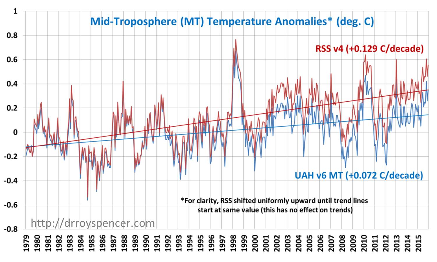
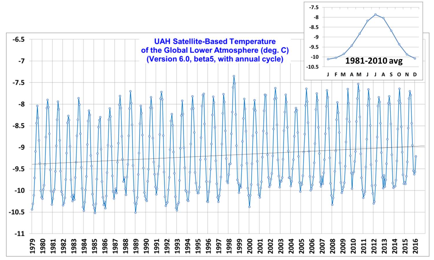
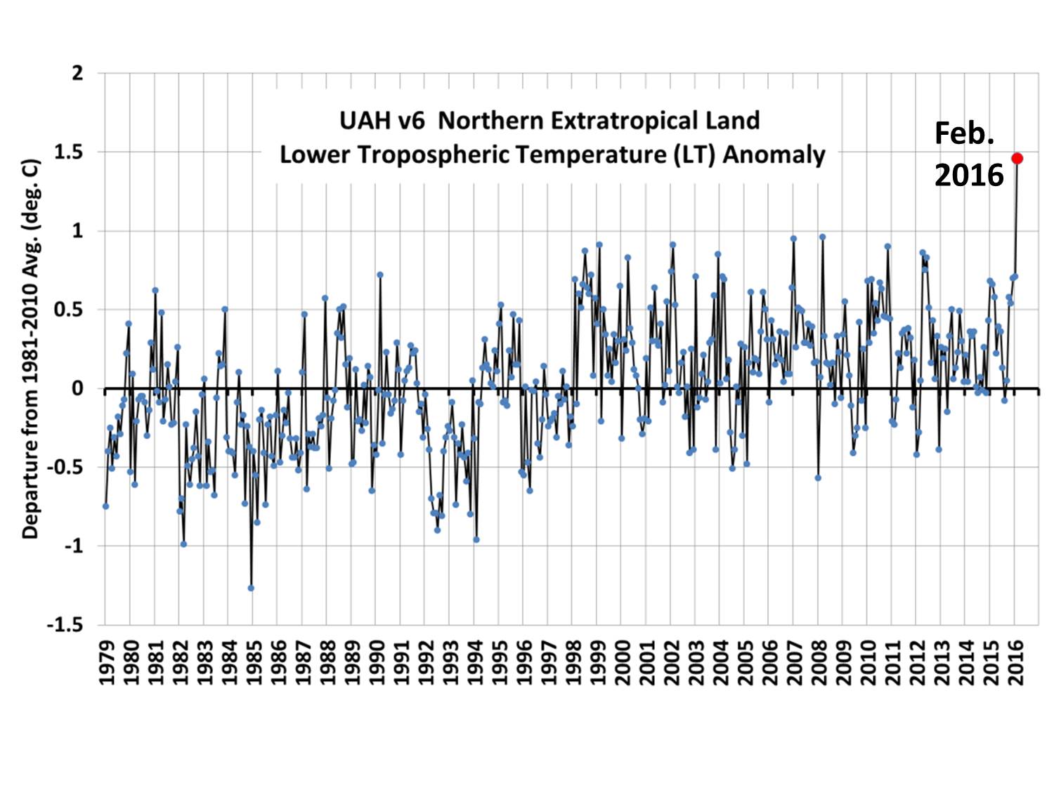
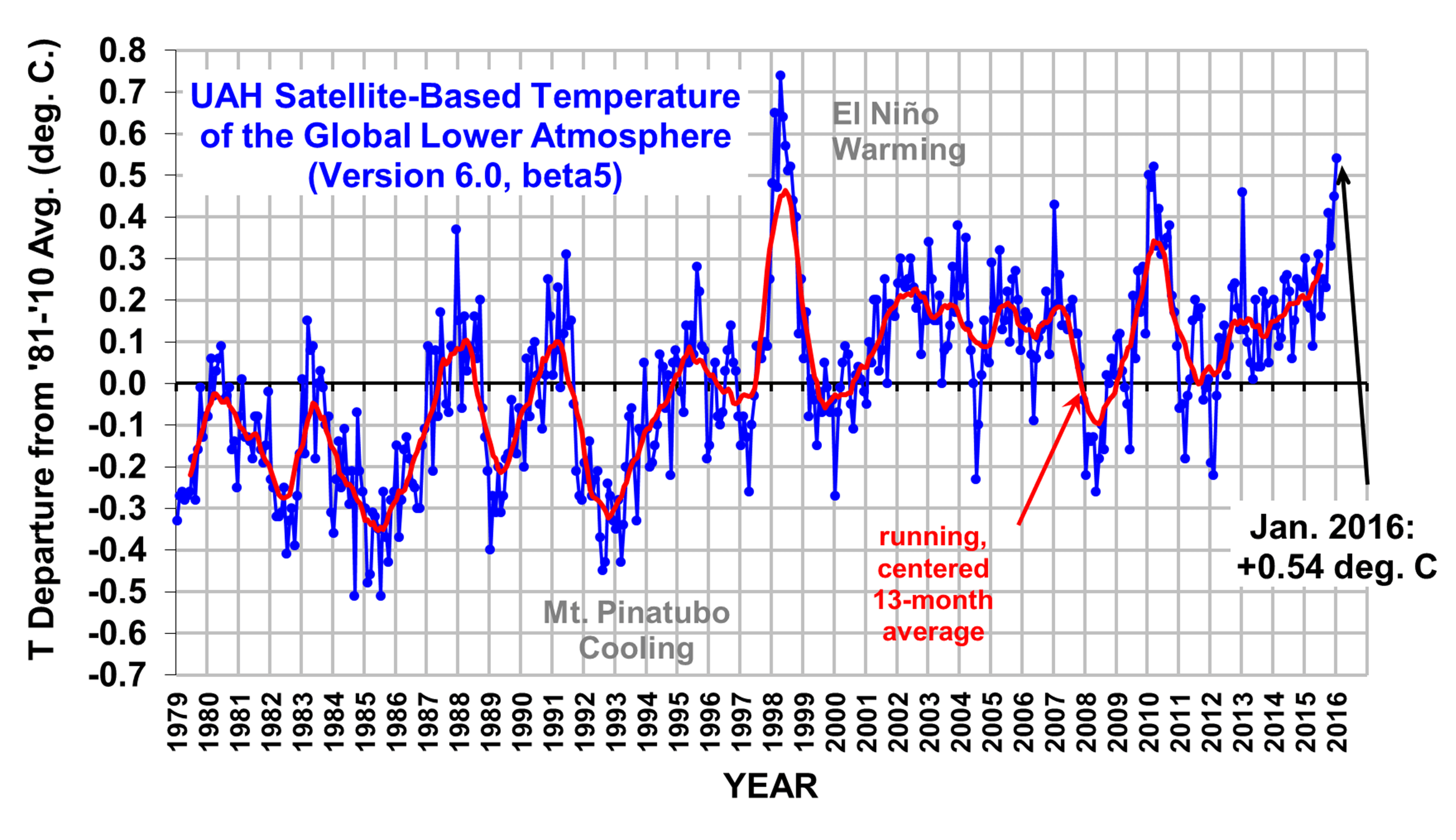
In contrast, our satellite analysis has 2015 only third warmest which has also been widely reported for weeks now. I understand that the RSS satellite analysis has it 4th warmest.
And yet I have had many e-mail requests to address the new reports of warmest year on record. I’ve been reluctant to because, well, this is all old news. (Also, my blog has been under almost constant “brute force login attacks” for the last month, from a variety of IP addresses, making posting nearly impossible most days).
There are many things I could say, but I would be repeating myself:
– Land measurements …that thermometers over land appear to have serious spurious warming issues from urbanization effects. Anthony Watts is to be credited for spearheading the effort to demonstrate this over the U.S. where recent warming has been exaggerated by about 60%, and I suspect the problem in other regions of the global will be at least as bad. Apparently, the NOAA homogenization procedure forces good data to match bad data. That the raw data has serious spurious warming effects is easy to demonstrate…and has been for the last 50 years in the peer-reviewed literature….why is it not yet explicitly estimated and removed?
– Ocean Measurements …that even some NOAA scientists don’t like the new Karlized ocean surface temperature dataset that made the global warming pause disappear; many feel it also forces good data to agree with bad data. (I see a common theme here.)
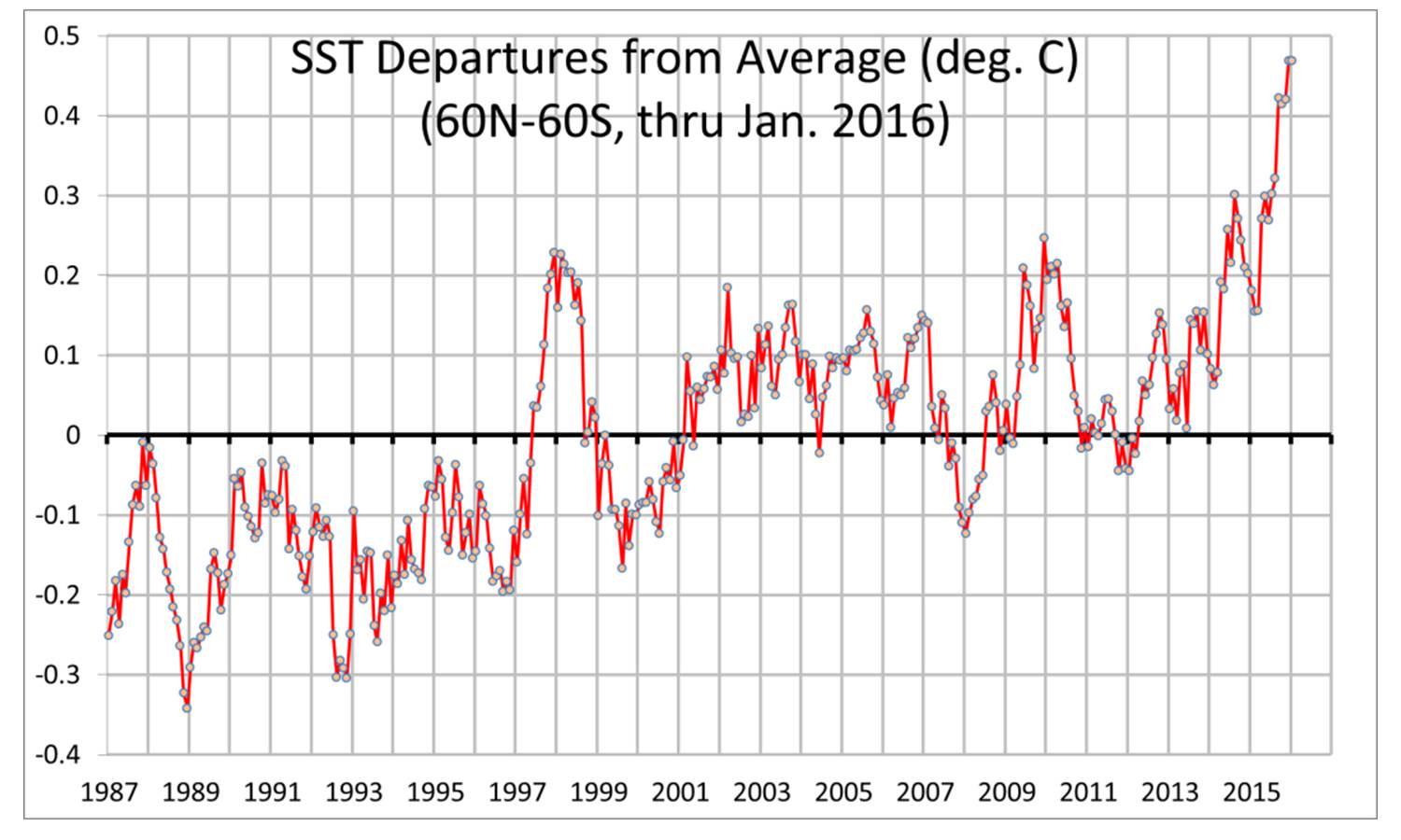
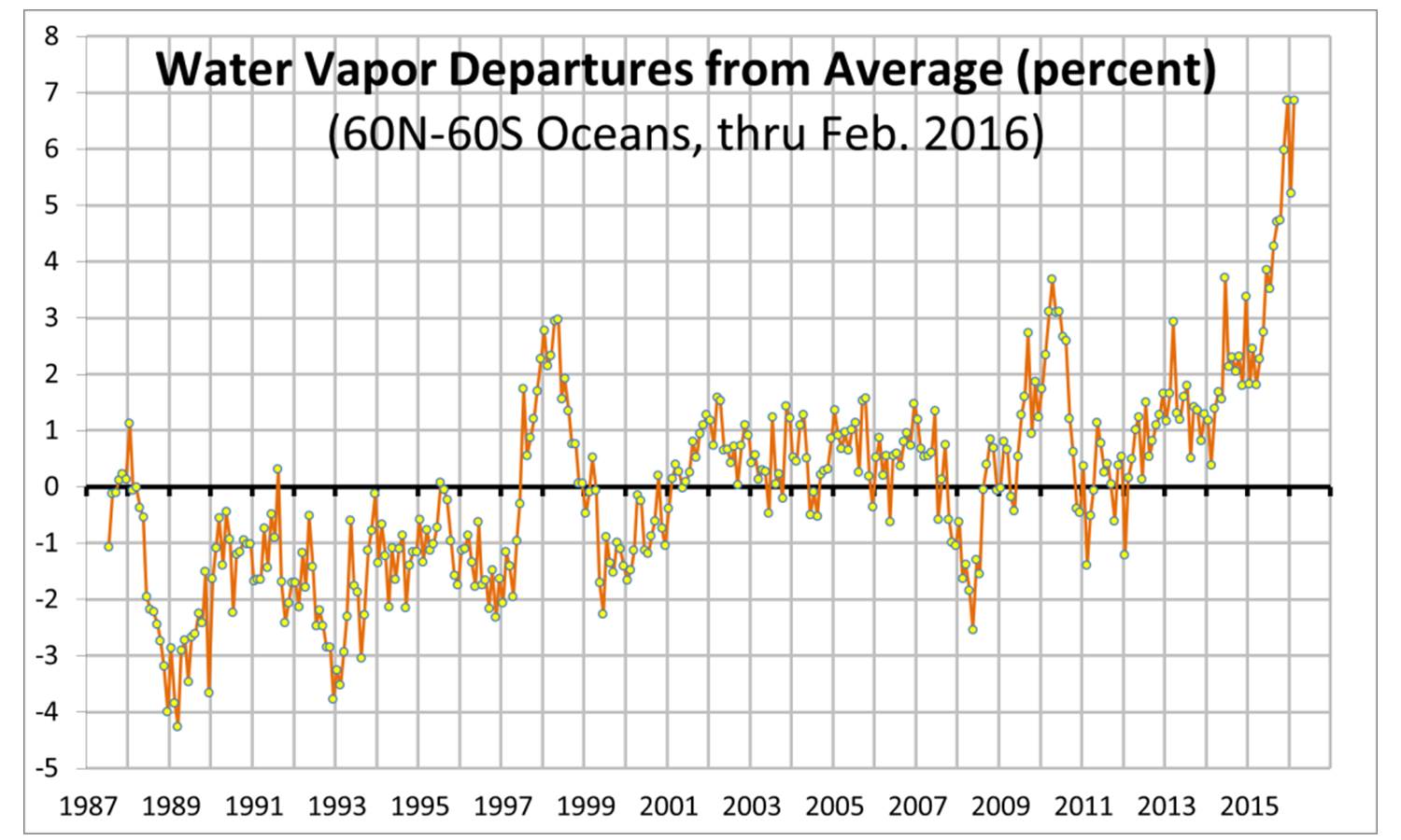
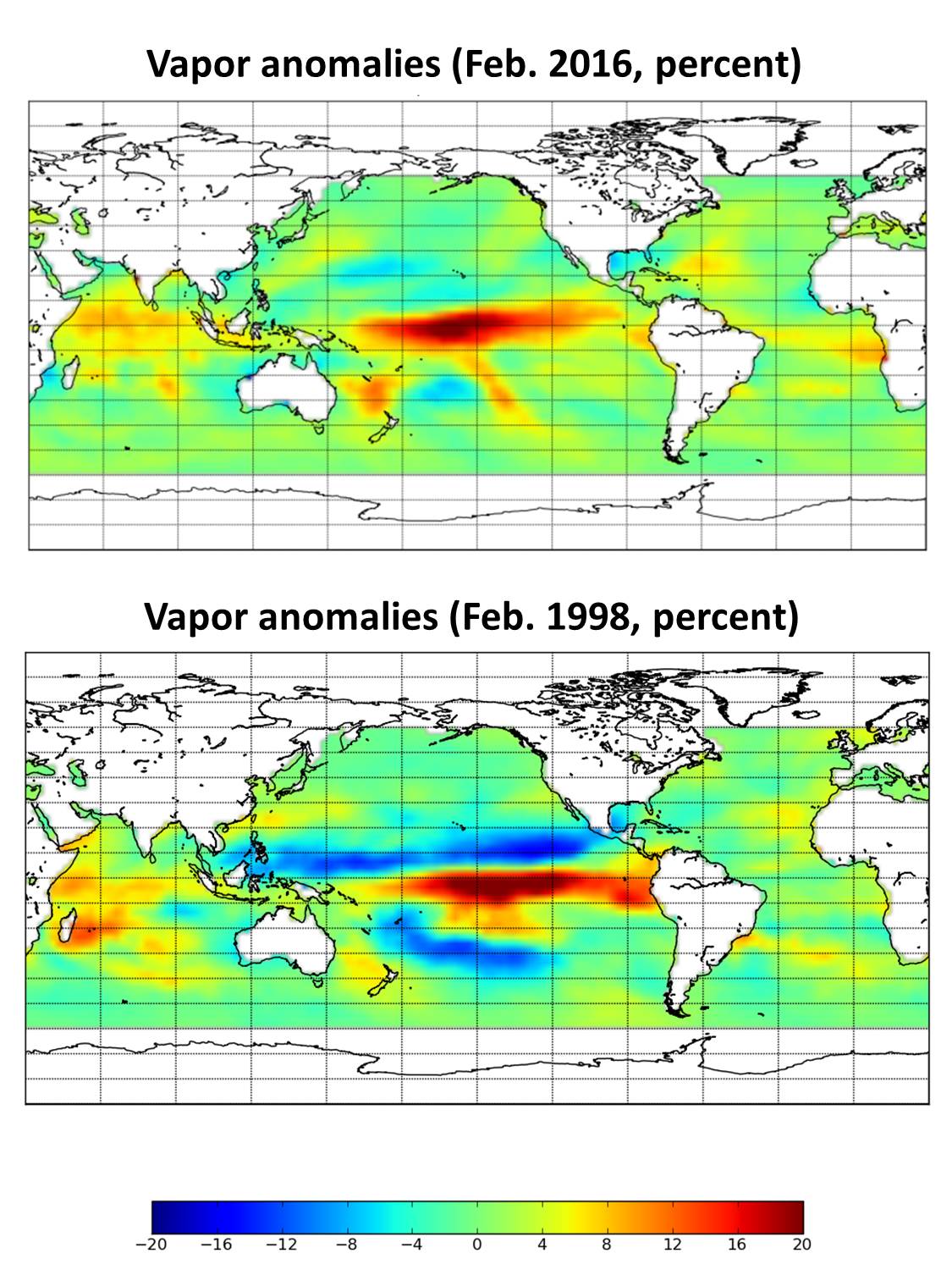
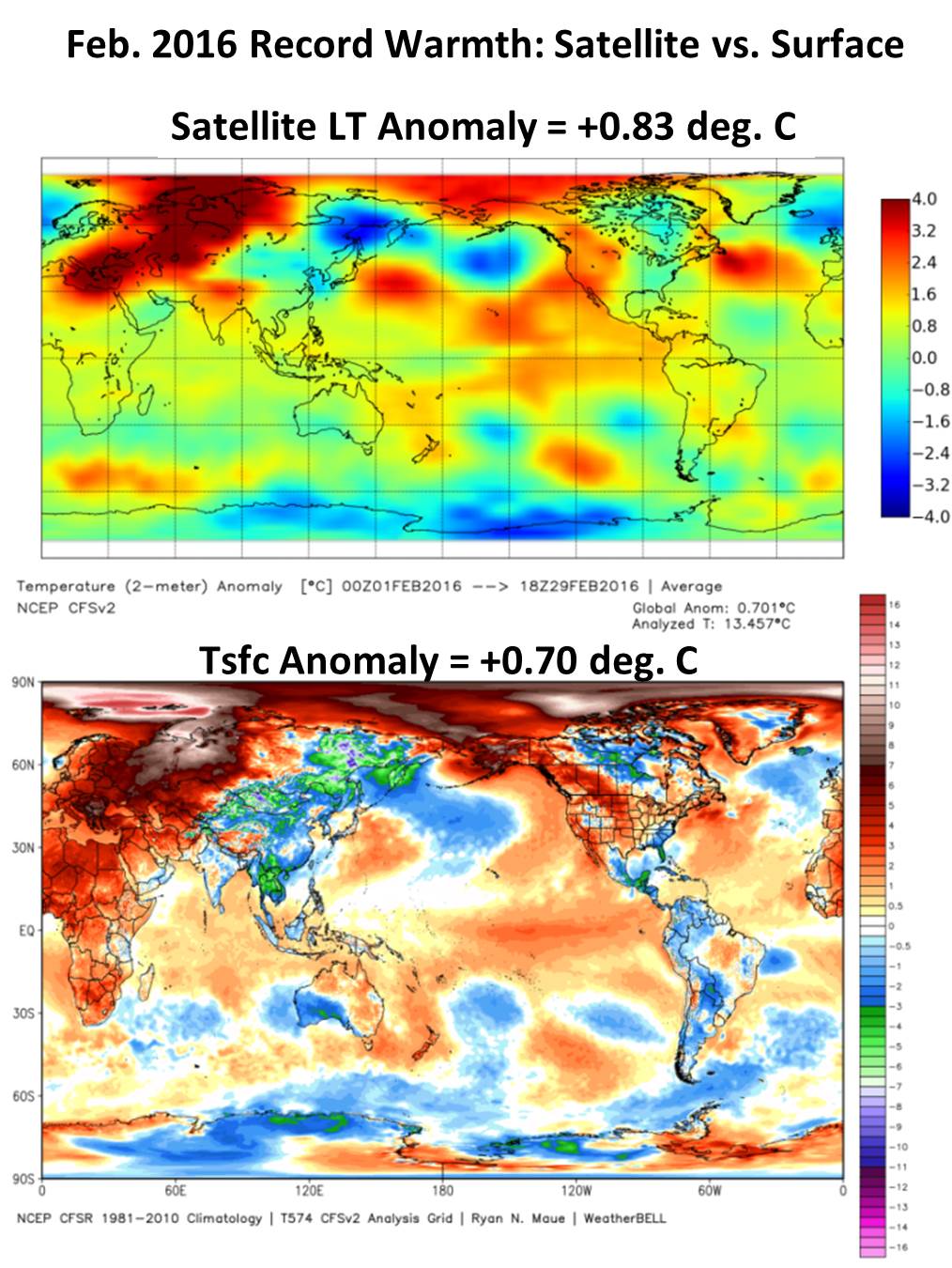
– El Nino …that a goodly portion of the record warmth in 2015 was naturally induced, just as it was in previous record warm years.
– Thermometers Still Disagree with Models …that even if 2015 is the warmest on record, and NOAA has exactly the right answer, it is still well below the average forecast of the IPCC’s climate models, and something very close to that average forms the basis for global warming policy. In other words, even if every successive year is a new record, it matters quite a lot just how much warming we are talking about.
Then we have scientists out there claiming silly things, like the satellites measure temperatures at atmospheric altitudes where people don’t live anyway, so we should ignore them.
Oh, really? Would those same scientists also claim we should ignore the ocean heat content measurements — also where nobody lives — even though that is supposedly the most important piece of evidence that heat is accumulating in the climate system?
Hmmm?
Finally, I don’t see why any of this matters anyway. Didn’t the Paris agreement in December signify that world governments are going to fix the global warming problem?
Or was that message oversold, too?
I’m not claiming our satellite dataset is necessarily the best global temperature dataset in terms of trends, even though I currently suspect it is closer to being accurate than the surface record — that will be for history to decide. The divergence in surface and satellite trends remains a mystery, and cannot (in my opinion) continue indefinitely if both happen to be largely correct.
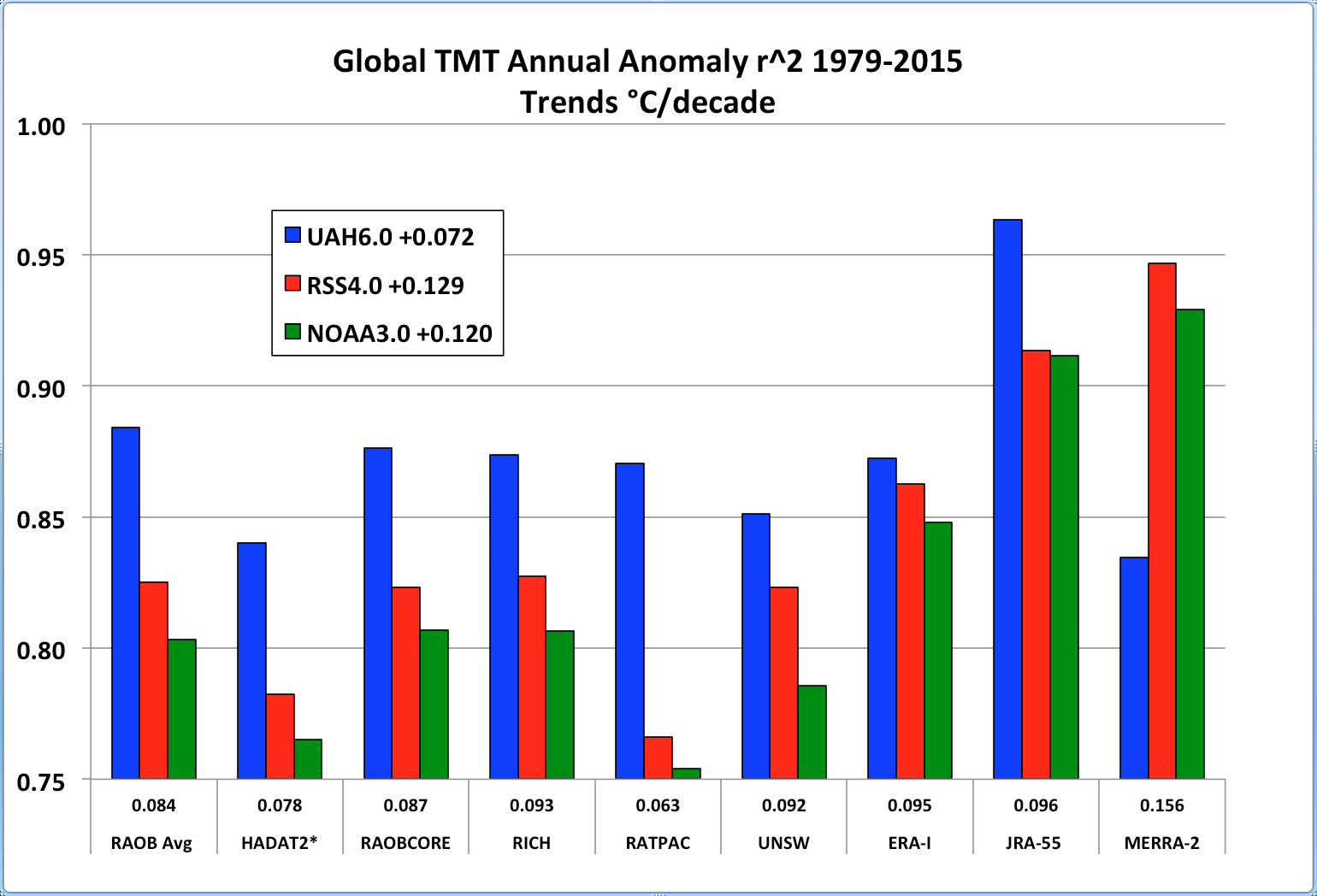
But since the satellites generally agree with (1) radiosondes and (2) most global reanalysis datasets (which use all observations radiosondes, surface temperatures, commercial aircraft, satellites, etc. everything except the kitchen sink), I think the fact that NOAA-NASA essentially ignores it reveals an institutional bias that the public who pays the bills is becoming increasingly aware of.
And this brings up the elephant in the room that I have a difficult time ignoring
By now it has become a truism that government agencies will prefer whichever dataset supports the governments desired policies. You might think that government agencies are only out to report the truth, but if that’s the case, why are these agencies run by political appointees?
I can say this as a former government employee who used to help NASA sell its programs to congress: We weren’t funded to investigate non-problems, and if global warming were ever to become a non-problem, funding would go away. I was told what I could and couldn’t say to Congress…Jim Hansen got to say whatever he wanted. I grew tired of it, and resigned.
Let me be clear: I’m not saying climate change is a non-problem; only that government programs that fund almost 100% of the research into climate change cannot be viewed as unbiased. Agencies can only maintain (or, preferable, grow) their budgets if the problem they want to study persists. Since at least the 1980s, an institutional bias exists which has encouraged the climate research community to view virtually all climate change as human-caused.
There indeed is a climate change problem to study…but I don’t think we know with any certainty how much is natural versus manmade. There is no way to know, because there is (contrary to the IPCC’s claims) no fingerprint of human versus natural warming. Even natural warming originating over the ocean will cause faster warming over land than over ocean, just as we already observe.
But since the government has framed virtually all of the research programs in terms of human-caused climate change, that’s what the funded scientists will dutifully report it to be, in terms of supposed causation.
And until the culture in the government funding agencies changes, I don’t see a new way of doing business materializing. It might require congress to direct the funding agencies to spend at least a small portion of their budgets to look for evidence of natural causes of climate change.
Because scientists, I have learned, will tend to find whatever they are paid to find in terms of causation…which is sometimes very difficult to pin down in science.

 Home/Blog
 The revelation that AG Loretta Lynch had discussions about bringing charges against climate change deniers (I’ve yet to meet a ‘climate change denier’) has led to a few questions about whether people like me (a skeptic of the view that the human influence on climate is either large or dangerous) should be worried.