My Global Warming Skepticism, for Dummies

July 17th, 2010

I receive many e-mails, and a recurring complaint is that many of my posts are too technical to understand. This morning’s installment arrived with the subject line, “Please Talk to Us”, and suggested I provide short, concise, easily understood summaries and explanations “for dummies”.

So, here’s a list of basic climate change questions, and brief answers based upon what I know today. I might update them as I receive suggestions and comments. I will also be adding links to other sources, and some visual aids, as appropriate.

Deja vu tells me I might have done this once before, but I’m too lazy to go back and see. So, I’ll start over from scratch. (Insert smiley)

It is important to understand at the outset that those of us who are skeptical of mankind’s influence on climate have a wide variety of views on the subject, and we can’t all be right. In fact, in this business, it is really easy to be wrong. It seems like everyone has a theory of what causes climate change. But it only takes one of us to be right for the IPCC’s anthropogenic global warming (AGW) house of cards to collapse.

As I like to say, taking measurements of the climate system is much easier than figuring out what those measurements mean in terms of cause and effect. Generally speaking, it’s not the warming that is in dispute…it’s the cause of the warming.

If you disagree with my views on something, please don’t flame me. Chances are, I’ve already heard your point of view; very seldom am I provided with new evidence I haven’t already taken into account.

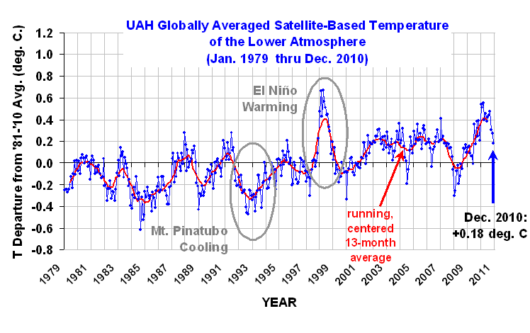
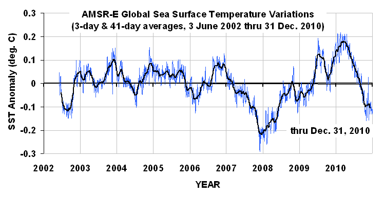
1) Are Global Temperatures Rising Now? There is no way to know, because natural year-to-year variability in global temperature is so large, with warming and cooling occurring all the time. What we can say is that surface and lower atmospheric temperature have risen in the last 30 to 50 years, with most of that warming in the Northern Hemisphere. Also, the magnitude of recent warming is somewhat uncertain, due to problems in making long-term temperature measurements with thermometers without those measurements being corrupted by a variety of non-climate effects. But there is no way to know if temperatures are continuing to rise now…we only see warming (or cooling) in the rearview mirror, when we look back in time.

2) Why Do Some Scientists Say It’s Cooling, while Others Say that Warming is Even Accelerating?
Since there is so much year-to-year (and even decade-to-decade) variability in global average temperatures, whether it has warmed or cooled depends upon how far back you look in time. For instance, over the last 100 years, there was an overall warming which was stronger toward the end of the 20th Century. This is why some say “warming is accelerating”. But if we look at a shorter, more recent period of time, say since the record warm year of 1998, one could say that it has cooled in the last 10-12 years. But, as I mentioned above, neither of these can tell us anything about whether warming is happening “now”, or will happen in the future.

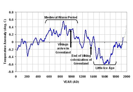
3) Haven’t Global Temperatures Risen Before? Yes. In the longer term, say hundreds to thousands of years, there is considerable indirect, proxy evidence (not from thermometers) of both warming and cooling. Since humankind can’t be responsible for these early events, this is evidence that nature can cause warming and cooling. If that is the case, it then opens up the possibility that some (or most) of the warming in the last 50 years has been natural, too. While many geologists like to point to much larger temperature changes are believed to have occurred over millions of years, I am unconvinced that this tells us anything of use for understanding how humans might influence climate on time scales of 10 to 100 years.

4) But Didn’t the “Hockey Stick” Show Recent Warming to be Unprecedented? The “hockey Stick” reconstructions of temperature variations over the last 1 to 2 thousand years have been a huge source of controversy. The hockey stick was previously used by the IPCC as a veritable poster child for anthropogenic warming, since it seemed to indicate there have been no substantial temperature changes over the last 1,000 to 2,000 years until humans got involved in the 20th Century. The various versions of the hockey stick were based upon limited amounts of temperature proxy evidence — primarily tree rings — and involved questionable statistical methods. In contrast, I think the bulk of the proxy evidence supports the view that it was at least as warm during the Medieval Warm Period, around 1000 AD. The very fact that recent tree ring data erroneously suggests cooling in the last 50 years, when in fact there has been warming, should be a warning flag about using tree ring data for figuring out how warm it was 1,000 years ago. But without actual thermometer data, we will never know for sure.

5) Isn’t the Melting of Arctic Sea Ice Evidence of Warming? Warming, yes…manmade warming, no. Arctic sea ice naturally melts back every summer, but that meltback was observed to reach a peak in 2007. But we have relatively accurate, satellite-based measurements of Arctic (and Antarctic) sea ice only since 1979. It is entirely possible that late summer Arctic Sea ice cover was just as low in the 1920s or 1930s, a period when Arctic thermometer data suggests it was just as warm. Unfortunately, there is no way to know, because we did not have satellites back then. Interestingly, Antarctic sea ice has been growing nearly as fast as Arctic ice has been melting over the last 30+ years.

6) What about rising sea levels? I must confess, I don’t pay much attention to the sea level issue. I will say that, to the extent that warming occurs, sea levels can be expected to also rise to some extent. The rise is partly due to thermal expansion of the water, and partly due to melting or shedding of land-locked ice (the Greenland and Antarctic ice sheets, and glaciers). But this says nothing about whether or not humans are the cause of that warming. Since there is evidence that glacier retreat and sea level rise started well before humans can be blamed, causation is — once again — a major source of uncertainty.

7) Is Increasing CO2 Even Capable of Causing Warming? There are some very intelligent people out there who claim that adding more carbon dioxide to the atmosphere can’t cause warming anyway. They claim things like, “the atmospheric CO2 absorption bands are already saturated”, or something else very technical. [And for those more technically-minded persons, yes, I agree that the effective radiating temperature of the Earth in the infrared is determined by how much sunlight is absorbed by the Earth. But that doesn’t mean the lower atmosphere cannot warm from adding more greenhouse gases, because at the same time they also cool the upper atmosphere]. While it is true that most of the CO2-caused warming in the atmosphere was there before humans ever started burning coal and driving SUVs, this is all taken into account by computerized climate models that predict global warming. Adding more “should” cause warming, with the magnitude of that warming being the real question. But I’m still open to the possibility that a major error has been made on this fundamental point. Stranger things have happened in science before.

8 ) Is Atmospheric CO2 Increasing? Yes, and most strongly in the last 50 years…which is why “most” climate researchers think the CO2 rise is the cause of the warming. Our site measurements of CO2 increase from around the world are possibly the most accurate long-term, climate-related, measurements in existence.

9) Are Humans Responsible for the CO2 Rise? While there are short-term (year-to-year) fluctuations in the atmospheric CO2 concentration due to natural causes, especially El Nino and La Nina, I currently believe that most of the long-term increase is probably due to our use of fossil fuels. But from what I can tell, the supposed “proof” of humans being the source of increasing CO2 — a change in the atmospheric concentration of the carbon isotope C13 — would also be consistent with a natural, biological source. The current atmospheric CO2 level is about 390 parts per million by volume, up from a pre-industrial level estimated to be around 270 ppm…maybe less. CO2 levels can be much higher in cities, and in buildings with people in them.

10) But Aren’t Natural CO2 Emissions About 20 Times the Human Emissions? Yes, but nature is believed to absorb CO2 at about the same rate it is produced. You can think of the reservoir of atmospheric CO2 as being like a giant container of water, with nature pumping in a steady stream into the bottom of the container (atmosphere) in some places, sucking out about the same amount in other places, and then humans causing a steady drip-drip-drip into the container. Significantly, about 50% of what we produce is sucked out of the atmosphere by nature, mostly through photosynthesis. Nature loves the stuff. CO2 is the elixir of life on Earth. Imagine the howls of protest there would be if we were destroying atmospheric CO2, rather than creating more of it.

11) Is Rising CO2 the Cause of Recent Warming? While this is theoretically possible, I think it is more likely that the warming is mostly natural. At the very least, we have no way of determining what proportion is natural versus human-caused.

12) Why Do Most Scientists Believe CO2 is Responsible for the Warming? Because (as they have told me) they can’t think of anything else that might have caused it. Significantly, it’s not that there is evidence nature can’t be the cause, but a lack of sufficiently accurate measurements to determine if nature is the cause. This is a hugely important distinction, and one the public and policymakers have been misled on by the IPCC.

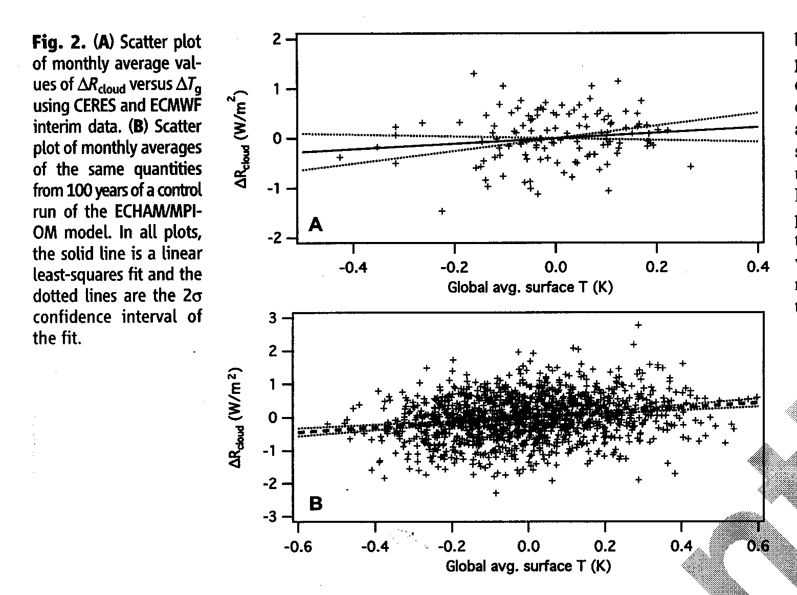
13) If Not Humans, What could Have Caused Recent Warming? This is one of my areas of research. I believe that natural changes in the amount of sunlight being absorbed by the Earth — due to natural changes in cloud cover — are responsible for most of the warming. Whether that is the specific mechanism or not, I advance the minority view that the climate system can change all by itself. Climate change does not require an “external” source of forcing, such as a change in the sun.

14) So, What Could Cause Natural Cloud Changes? I think small, long-term changes in atmospheric and oceanic flow patterns can cause ~1% changes in how much sunlight is let in by clouds to warm the Earth. This is all that is required to cause global warming or cooling. Unfortunately, we do not have sufficiently accurate cloud measurements to determine whether this is the primary cause of warming in the last 30 to 50 years.

15) How Significant is the Climategate Release of E-Mails? While Climategate does not, by itself, invalidate the IPCC’s case that global warming has happened, or that humans are the primary cause of that warming, it DOES illustrate something I emphasized in my first book, “Climate Confusion”: climate researchers are human, and prone to bias.

16) Why Would Bias in Climate Research be Important? I thought Scientists Just Follow the Data Where It Leads Them When researchers approach a problem, their pre-conceived notions often guide them. It’s not that the IPCC’s claim that humans cause global warming is somehow untenable or impossible, it’s that political and financial pressures have resulted in the IPCC almost totally ignoring alternative explanations for that warming.

17) How Important Is “Scientific Consensus” in Climate Research? In the case of global warming, it is nearly worthless. The climate system is so complex that the vast majority of climate scientists — usually experts in variety of specialized fields — assume there are more knowledgeable scientists, and they are just supporting the opinions of their colleagues. And among that small group of most knowledgeable experts, there is a considerable element of groupthink, herd mentality, peer pressure, political pressure, support of certain energy policies, and desire to Save the Earth — whether it needs to be saved or not.

18) How Important are Computerized Climate Models? I consider climate models as being our best way of exploring cause and effect in the climate system. It is really easy to be wrong in this business, and unless you can demonstrate causation with numbers in equations, you are stuck with scientists trying to persuade one another by waving their hands. Unfortunately, there is no guarantee that climate models will ever produce a useful prediction of the future. Nevertheless, we must use them, and we learn a lot from them. My biggest concern is that models have been used almost exclusively for supporting the claim that humans cause global warming, rather than for exploring alternative hypotheses — e.g. natural climate variations — as possible causes of that warming.

19) What Do I Predict for Global Temperature Changes in the Future? I tend to shy away from long-term predictions, because there are still so many uncertainties. When pressed, though, I tend to say that I think cooling in our future is just as real a possibility as warming. Of course, a third possibility is relatively steady temperatures, without significant long-term warming or cooling. Keep in mind that, while you will find out tomorrow whether your favorite weather forecaster is right or wrong, no one will remember 50 years from now a scientist today wrongly predicting we will all die from heat stroke by 2060.

Concluding Remarks

Climate researchers do not know nearly as much about the causes of climate change as they profess. We have a pretty good understanding of how the climate system works on average…but the reasons for small, long-term changes in climate system are still extremely uncertain.

The total amount of CO2 humans have added to the atmosphere in the last 100 years has upset the radiative energy budget of the Earth by only 1%. How the climate system responds to that small “poke” is very uncertain. The IPCC says there will be strong warming, with cloud changes making the warming worse. I claim there will be weak warming, with cloud changes acting to reduce the influence of that 1% change. The difference between these two outcomes is whether cloud feedbacks are positive (the IPCC view), or negative (the view I and a minority of others have).

So far, neither side has been able to prove their case. That uncertainty even exists on this core issue is not appreciated by many scientists!

Again I will emphasize, some very smart people who consider themselves skeptics will disagree with some of my views stated above, particularly when it involves explanations for what has caused warming, and what has caused atmospheric CO2 to increase.

Unlike the global marching army of climate researchers the IPCC has enlisted, we do not walk in lockstep. We are willing to admit, “we don’t really know”, rather than mislead people with phrases like, “the warming we see is consistent with an increase in CO2”, and then have the public think that means, “we have determined, through our extensive research into all the possibilities, that the warming cannot be due to anything but CO2”.

Skeptics advancing alternative explanations (hypotheses) for climate variability represent the way the researcher community used to operate, before politics, policy outcomes, and billions of dollars got involved.

WeatherShop.com Gifts, gadgets, weather stations, software and more...click here!

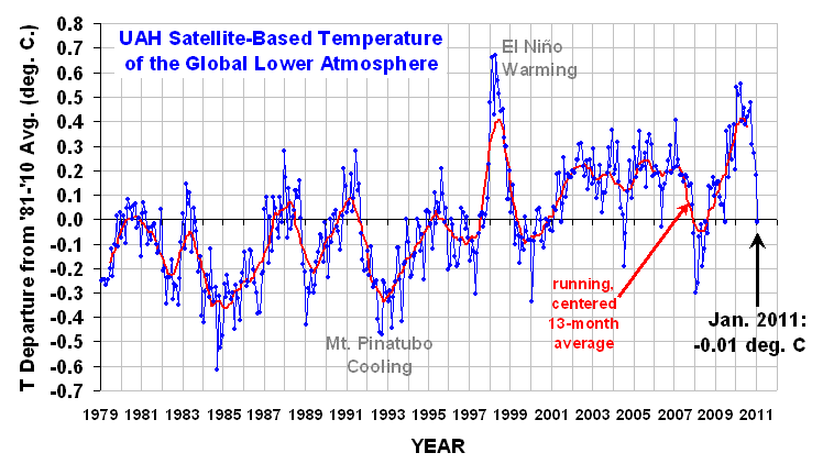
June 2010 UAH Global Temperature Update: +0.44 deg. C

July 1st, 2010


YR MON GLOBE NH SH TROPICS
2009 1 0.251 0.472 0.030 -0.068
2009 2 0.247 0.564 -0.071 -0.045
2009 3 0.191 0.324 0.058 -0.159
2009 4 0.162 0.316 0.008 0.012
2009 5 0.140 0.161 0.119 -0.059
2009 6 0.043 -0.017 0.103 0.110
2009 7 0.429 0.189 0.668 0.506
2009 8 0.242 0.235 0.248 0.406
2009 9 0.505 0.597 0.413 0.594
2009 10 0.362 0.332 0.393 0.383
2009 11 0.498 0.453 0.543 0.479
2009 12 0.284 0.358 0.211 0.506
2010 1 0.648 0.860 0.436 0.681
2010 2 0.603 0.720 0.486 0.791
2010 3 0.653 0.850 0.455 0.726
2010 4 0.501 0.799 0.203 0.633
2010 5 0.534 0.775 0.292 0.708
2010 6 0.436 0.552 0.321 0.475

UAH_LT_1979_thru_June_10

The global-average lower tropospheric temperature remains warm, +0.44 deg. C for June, 2010, but it appears the El Nino warmth is waning as a La Nina approaches.

For those keeping track of whether 2010 ends up being a record warm year, 1998 still leads with the daily average for 1 Jan to 30 June being +0.64 C in 1998 compared with +0.56 C for 2010. (John Christy says that the difference is not statistically significant.) As of 30 June 2010, there have been 181 days in the year. From our calibrated daily data, we find that 1998 was warmer than 2010 on 122 (two-thirds) of them.

As a reminder, four months ago we changed to Version 5.3 of our dataset, which accounts for the mismatch between the average seasonal cycle produced by the older MSU and the newer AMSU instruments. This affects the value of the individual monthly departures, but does not affect the year to year variations, and thus the overall trend remains the same as in Version 5.2. ALSO…we have added the NOAA-18 AMSU to the data processing in v5.3, which provides data since June of 2005. The local observation time of NOAA-18 (now close to 2 p.m., ascending node) is similar to that of NASA’s Aqua satellite (about 1:30 p.m.). The temperature anomalies listed above have changed somewhat as a result of adding NOAA-18.

[NOTE: These satellite measurements are not calibrated to surface thermometer data in any way, but instead use on-board redundant precision platinum resistance thermometers (PRTs) carried on the satellite radiometers. The PRT’s are individually calibrated in a laboratory before being installed in the instruments.]


Revisiting the Pinatubo Eruption as a Test of Climate Sensitivity

June 23rd, 2010


The eruption of Mt. Pinatubo in the Philippines on June 15, 1991 provided a natural test of the climate system to radiative forcing by producing substantial cooling of global average temperatures over a period of 1 to 2 years. There have been many papers which have studied the event in an attempt to determine the sensitivity of the climate system, so that we might reduce the (currently large) uncertainty in the future magnitude of anthropogenic global warming.

In perusing some of these papers, I find that the issue has been made unnecessarily complicated and obscure. I think part of the problem is that too many investigators have tried to approach the problem from the paradigm most of us have been misled by: believing that sensitivity can be estimated from the difference between two equilibrium climate states, say before the Pinatubo eruption, and then as the climate system responds to the Pinatubo aerosols. The trouble is that this is not possible unless the forcing remains constant, which clearly is not the case since most of the Pinatubo aerosols are gone after about 2 years.

Here I will briefly address the pertinent issues, and show what I believe to be the simplest explanation of what can — and cannot — be gleaned from the post-eruption response of the climate system. And, in the process, we will find that the climate system’s response to Pinatubo might not support the relatively high climate sensitivity that many investigators claim.

Radiative Forcing Versus Feedback
I will once again return to the simple model of the climate system’s average change in temperature from an equilibrium state. Some call it the “heat balance equation”, and it is concise, elegant, and powerful. To my knowledge, no one has shown why such a simple model can not capture the essence of the climate system’s response to an event like the Pinatubo eruption. Increased complexity does not necessarily ensure increased accuracy.

The simple model can be expressed in words as:

[system heat capacity] x[temperature change with time] = [Radiative Forcing] – [Radiative Feedback],

or with mathematical symbols as:

Cp*[dT/dt] = F – lambda*T .

Basically, this equation says that the temperature change with time [dT/dt] of a climate system with a certain heat capacity [Cp, dominated by the ocean depth over which heat is mixed] is equal to the radiative forcing [F] imposed upon the system minus any radiative feedback [lambda*T] upon the resulting temperature change. (The left side is also equivalent to the change in the heat content of the system with time.)

The feedback parameter (lambda, always a positive number if the above equation is expressed with a negative sign) is what we are interested in determining, because its reciprocal is the climate sensitivity. The net radiative feedback is what “tries” to restore the system temperature back to an equilibrium state.

Lambda represents the combined effect of all feedbacks PLUS the dominating, direct infrared (Planck) response to increasing temperature. This Planck response is estimated to be 3.3 Watts per sq. meter per degree C for the average effective radiating temperature of the Earth, 255K. Clouds, water vapor, and other feedbacks either reduce the total “restoring force” to below 3.3 (positive feedbacks dominate), or increase it above 3.3 (negative feedbacks dominate).

Note that even though the Planck effect behaves like a strong negative feedback, and is even included in the net feedback parameter, for some reason it is not included in the list of climate feedbacks. This is probably just to further confuse us.

If positive feedbacks were strong enough to cause the net feedback parameter to go negative, the climate system would potentially be unstable to temperature changes forced upon it. For reference, all 21 IPCC climate models exhibit modest positive feedbacks, with lambda ranging from 0.8 to 1.8 Watts per sq. meter per degree C, so none of them are inherently unstable.

This simple model captures the two most important processes in global-average temperature variability: (1) through energy conservation, it translates a global, top-of-atmosphere radiative energy imbalance into a temperature change of a uniformly mixed layer of water; and (2) a radiative feedback restoring forcing in response to that temperature change, the value of which depends upon the sum of all feedbacks in the climate system.


Modeling the Post-Pinatubo Temperature Response

So how do we use the above equation together with measurements of the climate system to estimate the feedback parameter, lambda? Well, let’s start with 2 important global measurements we have from satellites during that period:

1) ERBE (Earth Radiation Budget Experiment) measurements of the variations in the Earth’s radiative energy balance, and

2) the change in global average temperature with time [dT/dt] of the lower troposphere from the satellite MSU (Microwave Sounding Unit) instruments.

Importantly — and contrary to common beliefs – the ERBE measurements of radiative imbalance do NOT represent radiative forcing. They instead represent the entire right hand side of the above equation: a sum of radiative forcing AND radiative feedback, in unknown proportions.

In fact, this net radiative imbalance (forcing + feedback) is all we need to know to estimate one of the unknowns: the system net heat capacity, Cp. The following two plots show for the pre- and post-Pinatubo period (a) the ERBE radiative balance variations; and (b) the MSU tropospheric temperature variations, along with 3 model simulations using the above equation. [The ERBE radiative flux measurements are necessarily 72-day averages to match the satellite’s orbit precession rate, so I have also computed 72-day temperature averages from the MSU, and run the model with a 72-day time step].

As can be seen in panel b, the MSU-observed temperature variations are consistent with a heat capacity equivalent to an ocean mixed layer depth of about 40 meters.

So, What is the Climate Model’s Sensitivity, Roy?
I think this is where confusion usually enters the picture. In running the above model, note that it was not necessary to assume a value for lambda, the net feedback parameter. In other words, the above model simulation did not depend upon climate sensitivity at all!

Again, I will emphasize: Modeling the observed temperature response of the climate system based only upon ERBE-measured radiative imbalances does not require any assumption regarding climate sensitivity. All we need to know was how much extra radiant energy the Earth was losing [or gaining], which is what the ERBE measurements represent.

Conceptually, the global-average ERBE-measured radiative imbalances measured after the Pinatubo eruption are some combination of (1) radiative forcing from the Pinatubo aerosols, and (2) net radiative feedback upon the resulting temperature changes opposing the temperature changes resulting from that forcing– but we do not know how much of each. There are an infinite number of combinations of forcing and feedback that would be able to explain the satellite observations.

Nevertheless, we do know ONE difference in how forcing and feedback are expressed over time: Temperature changes lag the radiative forcing, but radiative feedback is simultaneous with temperature change.

What we need to separate the two is another source of information to sort out how much forcing versus feedback is involved, for instance something related to the time history of the radiative forcing from the volcanic aerosols. Otherwise, we can not use satellite measurements to determine net feedback in response to radiative forcing.

Fortunately, there is a totally independent satellite estimate of the radiative forcing from Pinatubo.

SAGE Estimates of the Pinatubo Aerosols
For anyone paying attention back then, the 1991 eruption of Pinatubo produced over one year of milky skies just before sunrise and just after sunset, as the sun lit up the stratospheric aerosols, composed mainly of sulfuric acid. The following photo was taken from the Space Shuttle during this time:

There are monthly stratospheric aerosol optical depth (tau) estimates archived at GISS, which during the Pinatubo period of time come from the SAGE (Stratospheric Aerosol and Gas Experiment). The following plot shows these monthly optical depth estimates for the same period of time we have been examining.

Note in the upper panel that the aerosols dissipated to about 50% of their peak concentration by the end of 1992, which is 18 months after the eruption. But look at the ERBE radiative imbalances in the bottom panel – the radiative imbalances at the end of 1992 are close to zero.

But how could the radiative imbalance of the Earth be close to zero at the end of 1992, when the aerosol optical depth is still at 50% of its peak?

The answer is that net radiative feedback is approximately canceling out the radiative forcing by the end of 1992. Persistent forcing of the climate system leads to a lagged – and growing – temperature response. Then, the larger the temperature response, the greater the radiative feedback which is opposing the radiative forcing as the system tries to restore equilibrium. (The climate system never actually reaches equilibrium, because it is always being perturbed by internal and external forcings…but, through feedback, it is always trying).

A Simple and Direct Feedback Estimate
Previous workers (e.g. Hansen et al., 2002) have calculated that the radiative forcing from the Pinatubo aerosols can be estimated directly from the aerosol optical depths measured by SAGE: the forcing in Watts per sq. meter is simply 21 times the optical depth.

Now we have sufficient information to estimate the net feedback. We simply subtract the SAGE-based estimates of Pinatubo radiative forcings from the ERBE net radiation variations (which are a sum of forcing and feedback), which should then yield radiative feedback estimates. We then compare those to the MSU lower tropospheric temperature variations to get an estimate of the feedback parameter, lambda. The data (after I have converted the SAGE monthly data to 72 day averages), looks like this:

The slope of 3.66 Watts per sq. meter per degree corresponds to weakly negative net feedback. If this corresponded to the feedback operating in response to increasing carbon dioxide concentrations, then doubling of atmosphere CO2 (2XCO2) would cause only 1 deg. C of warming. This is below the 1.5 deg. C lower limit the IPCC is 90% sure the climate sensitivity will not be below.

The Time History of Forcing and Feedback from Pinatubo
It is useful to see what two different estimates of the Pinatubo forcing looks like: (1) the direct estimate from SAGE, and (2) an indirect estimate from ERBE minus the MSU-estimated feedbacks, using our estimate of lambda = 3.66 Watts per sq. meter per deg. C. This is shown in the next plot:

Note that at the end of 1992, the Pinatubo aerosol forcing, which has decreased to about 50% of its peak value, almost exactly offsets the feedback, which has grown in proportion to the temperature anomaly. This is why the ERBE-measured radiative imbalance is close to zero…radiative feedback is canceling out the radiative forcing.

The reason why the ‘indirect’ forcing estimate looks different from the more direct SAGE-deduced forcing in the above figure is because there are other, internally-generated radiative “forcings” in the climate system measured by ERBE, probably due to natural cloud variations. In contrast, SAGE is a limb occultation instrument, which measures the aerosol loading of the cloud-free stratosphere when the instrument looks at the sun just above the Earth’s limb.

Discussion
I have shown that Earth radiation budget measurements together with global average temperatures can not be used to infer climate sensitivity (net feedback) in response to radiative forcing of the climate system. The only exception would be from the difference between two equilibrium climate states involving radiative forcing that is instantaneously imposed, and then remains constant over time. Only in this instance is all of the radiative variability due to feedback, not forcing.

Unfortunately, even though this hypothetical case has formed the basis for many investigations of climate sensitivity, this exception never happens in the real climate system

In the real world, some additional information is required regarding the time history of the forcing — preferably the forcing history itself. Otherwise, there are an infinite number of combinations of forcing and feedback which can explain a given set of satellite measurements of radiative flux variations and global temperature variations.

I currently believe the above methodology, or something similar, is the most direct way to estimate net feedback from satellite measurements of the climate system as it responds to a radiative forcing event like the Pinatubo eruption. The method is not new, as it is basically the same one used by Forster and Taylor (2006 J. of Climate) to estimate feedbacks in the IPCC AR4 climate models. Forster and Taylor took the global radiative imbalances the models produced over time (analogous to our ERBE measurements of the Earth), subtracted the radiative forcings that were imposed upon the models (usually increasing CO2), and then compared the resulting radiative feedback estimates to the corresponding temperature variations, just as I did in the scatter diagram above.

All I have done is apply the same methodology to the Pinatubo event. In fact, Forster and Gregory (also 2006 J. Climate) performed a similar analysis of the Pinatubo period, but for some reason got a feedback estimate closer to the IPCC climate models. I am using tropospheric temperatures, rather than surface temperatures as they did, but the 30+ year satellite record shows that year-to-year variations in tropospheric temperatures are larger than the surface temperatures variations. This means the feedback parameter estimated here (3.66) would be even larger if scaled to surface temperature. So, other than the fact that the ERBE data have relatively recently been recalibrated, I do not know why their results should differ so much from my results.

WeatherShop.com Gifts, gadgets, weather stations, software and more...click here!

The Global Warming Inquisition Has Begun

June 22nd, 2010


A new “study” has been published in the Proceedings of the National Academy of Sciences (PNAS) which has examined the credentials and publication records of climate scientists who are global warming skeptics versus those who accept the “tenets of anthropogenic climate change”.

Not surprisingly, the study finds that the skeptical scientists have fewer publications or are less credentialed than the marching army of scientists who have been paid hundreds of millions of dollars over the last 20 years to find every potential connection between fossil fuel use and changes in nature.

After all, nature does not cause change by itself, you know.

The study lends a pseudo-scientific air of respectability to what amounts to a black list of the minority of scientists who do not accept the premise that global warming is mostly the result of you driving your SUV and using incandescent light bulbs.

There is no question that there are very many more scientific papers which accept the mainstream view of global warming being caused by humans. And that might account for something if those papers actually independently investigated alternative, natural mechanisms that might explain most global warming in the last 30 to 50 years, and found that those natural mechanisms could not.

As just one of many alternative explanations, most of the warming we have measured in the last 30 years could have been caused by a natural, 2% decrease in cloud cover. Unfortunately, our measurements of global cloud cover over that time are nowhere near accurate enough to document such a change.

But those scientific studies did not address all of the alternative explanations. They couldn’t, because we do not have the data to investigate them. The vast majority of them simply assumed global warming was manmade.

I’m sorry, but in science a presupposition is not “evidence”.

Instead, anthropogenic climate change has become a scientific faith. The fact that the very first sentence in the PNAS article uses the phrase “tenets of anthropogenic climate change” hints at this, since the term “tenet” is most often used when referring to religious doctrine, or beliefs which cannot be proved to be true.

So, since we have no other evidence to go on, let’s pin the rap on humanity. It just so happens that’s the position politicians want, which is why politics played such a key role in the formation of the IPCC two decades ago.

The growing backlash against us skeptics makes me think of the Roman Catholic Inquisition, which started in the 12th Century. Of course, no one (I hope no one) will be tried and executed for not believing in anthropogenic climate change. But the fact that one of the five keywords or phrases attached to the new PNAS study is “climate denier” means that such divisive rhetoric is now considered to be part of our mainstream scientific lexicon by our country’s premier scientific organization, the National Academy of Sciences.

Surely, equating a belief in natural climate change to the belief that the Holocaust slaughter of millions of Jews and others by the Nazis never occurred is a new low for science as a discipline.

The new paper also implicitly adds most of the public to the black list, since surveys have shown dwindling public belief in the consensus view of climate change.

At least I have lots of company.

WeatherShop.com Gifts, gadgets, weather stations, software and more...click here!

Global Average Sea Surface Temperatures Continue their Plunge

June 18th, 2010

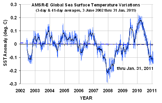
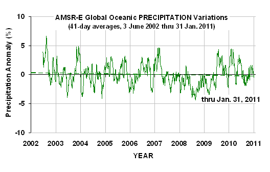
Sea Surface Temperatures (SSTs) measured by the AMSR-E instrument on NASA’s Aqua satellite continue their plunge as a predicted La Nina approaches. The following plot, updated through yesterday (June 17, 2010) shows that the cooling in the Nino34 region in the tropical east Pacific is well ahead of the cooling in the global average SST, something we did not see during the 2007-08 La Nina event (click on it for the large, undistorted version):

The rate at which the Nino34 SSTs are falling is particularly striking, as seen in this plot of the SST change rate for that region:

To give some idea of what is causing the global-average SST to fall so rapidly, I came up with an estimate of the change in reflected sunlight (shortwave, or SW flux) using our AMSR-E total integrated cloud water amounts. This was done with a 7+ year comparison of those cloud water estimates to daily global-ocean SW anomalies computed from the CERES radiation budget instrument, also on Aqua:

What this shows is an unusually large increase in reflected sunlight over the last several months, probably due to an increase in low cloud cover.

At this pace of cooling, I suspect that the second half of 2010 could ruin the chances of getting a record high global temperature for this year. Oh, darn.


FAQ #271: If Greenhouse Gases are such a Small Part of the Atmosphere, How Do They Change Its Temperature?

June 17th, 2010

NOTE posted 9:20 a.m. CDT 21 June, 2010: Upon reading the comments here, its obvious some have misinterpreted what I am discussing here. It’s NOT why greenhouse gases act to warm the lower atmosphere, it’s why a given parcel of air containing a very small fraction of greenhouse gases can be thoroughly warmed (or cooled, if in the upper atmosphere) by them.

Some of the questions I receive from the public tend to show up repeatedly. One of those more common questions I receive arrived once again yesterday, from a airplane pilot, who asked “If greenhouse gases are such a small proportion of the atmosphere,” (only 39 out of every 100,000 molecules are CO2), “how can they heat or cool all the rest of the air?”

The answer comes from the “kinetic theory of gases”. In effect, each CO2 molecule is a tiny heater (or air conditioner) depending on whether it is absorbing more infrared photons than it is emitting, or vice versa.

When the radiatively active molecules in the atmosphere — mainly water vapor, CO2, and methane — are heated by infrared radiation, even though they are a very small fraction of the total, they are moving very fast and do not have to travel very far before they collide with other molecules of air…that’s when they transfer part of their thermal energy to another molecule. That transfer is in the form of momentum from the molecule’s mass and its speed.

That molecule then bumps into others, those bump into still more, and on and on ad infinitum.

To give some idea of how fast all this happens, consider:

1) there are 26,900,000,000,000,000,000,000,000 molecules in 1 cubic meter of air at sea level.

2) at room temperature, each molecule is traveling at a very high speed, averaging 1,000 mph for heavier molecules like nitrogen, over 3,000 mph for the lightest molecule, hydrogen, etc.

3) the average distance a molecule travels before hitting another molecule (called the “mean free path”) is only 0.000067 of a millimeter

So, there are so many molecules traveling so fast, and so close to one another, that the radiatively active molecules almost instantly transfer any extra thermal energy (their velocity is proportional to the square root of their temperature) to other molecules. Or, if they happen to be cooling the air, the absorb extra momentum from the other air molecules.

From the above numbers we can compute that a single nitrogen molecule (air is mostly nitrogen) undergoes over 7 billion collisions every second.

All of this happens on extremely small scales, with gazillions of the radiatively active molecules scattered through a very small volume of air.

It is rather amazing that these relatively few “greenhouse” gases are largely responsible for the temperature structure of the atmosphere. Without them, the atmosphere would have no way of losing the heat energy that it gains from the Earth’s surface in response to solar heating.

Such an atmosphere would eventually become the same temperature throughout its depth, called an “isothermal” atmosphere. All vertical air motions would stop in such an atmosphere, which means there would be no weather either.

Now, I will have to endure the rash of e-mails I always get from those who do not believe that greenhouse gases do all of this. But that issue will have to be the subject of a later FAQ.

WeatherShop.com Gifts, gadgets, weather stations, software and more...click here!

Update on the Role of the Pacific Decadal Oscillation in Global Warming

June 17th, 2010

UPDATE: more edits & enhancements for clarity made at 3:35 CDT, June 17, 2010.

I’ve returned to the issue of determining to what extent the Pacific Decadal Oscillation (PDO) can at least partly explain global average temperature variations, including warming, during the 20th Century. We tried publishing a paper on this over a year ago and were immediately and swiftly rejected in a matter of days by a single (!) reviewer.

Here I use a simple forcing-feedback model, combined with satellite estimates of cloud changes caused by the PDO, to demonstrate the ability of the model to explain the temperature variations. This time, though, I am going to use Jim Hansen’s (GISS) record of yearly radiative forcings of the global climate system since 1900 to demonstrate more convincingly the importance of the PDO…not only for explaining the global temperature record of the past, but for the estimation of the sensitivity of the climate system and thus project the amount of future global warming (er, I mean climate change).

What follows is not meant to be publishable in a peer-reviewed paper. It is to keep the public informed, to stimulate discussion, to provide additional support for the claims in my latest book, and to help me better understand what I know at this point in my research, what I don’t know, and what direction I should go next.

The Simple Climate Model
I’m still using a simple forcing feedback-model of temperature variations, but have found that more than a single ocean layer is required to mimic both the faster time scales (e.g. 5-year) temperature fluctuations, while allowing a slower temperature response on multi-decadal time scales as heat diffuses from the upper ocean to the deeper ocean. The following diagram shows the main components of the model.

For forcing, I am assuming the GISS record of yearly-average forcing, the values of which I have plotted for the period since 1900 in the following graph:

I will simply assume these forcings are correct, and will show what happens in the model when I use: (1) all the GISS forcings together; (2) all GISS forcings except tropospheric aerosols, and (3) all the GISS forcings, but replacing the tropospheric aerosols with the satellite-derived PDO forcings.

Internal Radiative Forcing from the PDO
As readers here are well aware, I believe that there are internal modes of climate variability which can cause “internal radiative forcing” of the climate system. These would most easily be explained as circulation-induced changes in cloud cover. My leading candidate for this mechanism continues to be the Pacific Decadal Oscillation.

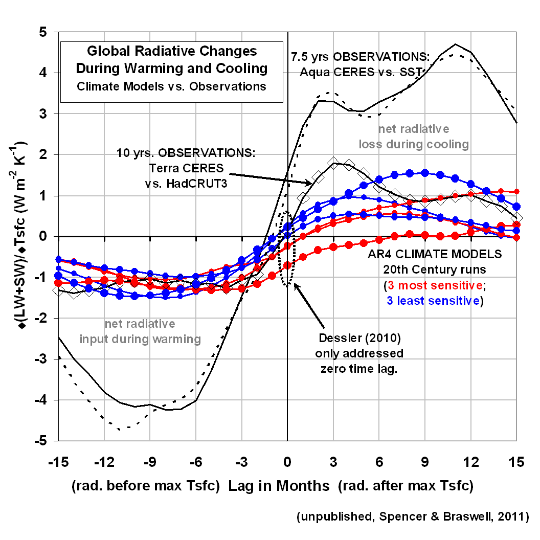
We have estimated the radiative forcing associated with the PDO by comparing yearly global averages of them to similar averages of CERES radiative flux variations over the Terra CERES period of record, 2000-2009. But since the CERES-measured radiative imbalances are a combination of forcing and feedback, we must remove an estimate of the feedback to get at the PDO forcing. [This step is completely consistent with, and analogous to, previous investigators removing known radiative forcings from climate model output in order to estimate feedbacks in those models].

Our new JGR paper (still awaiting publication) shows evidence that, for year-to-year climate variability at least, net feedback is about 6 Watts per sq. meter per degree C. After removal of the feedback component with our AMSU-based tropospheric temperature anomalies, the resulting relationship between yearly-running 3-year average PDO index versus radiative forcing looks like this:

This internally-generated radiative forcing is most likely due to changes in global average cloud cover associated with the PDO. If we apply this relationship to yearly estimates of the PDO index, we get the following estimate of “internal radiative forcing” from the PDO since 1900:

As can be seen, these radiative forcings – if they existed during the 20th Century– are comparable to the magnitude of the GISS forcings.

Model Simulations

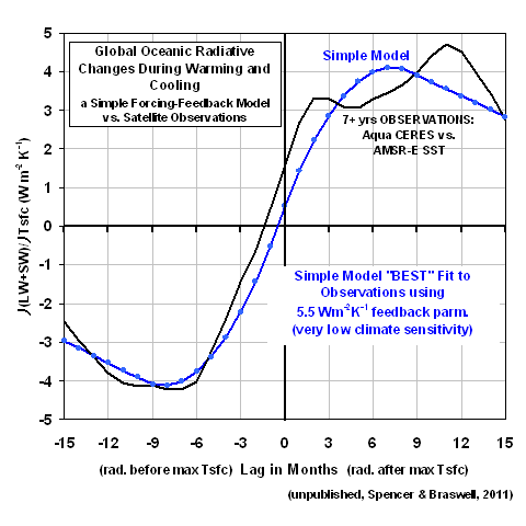
The model has 7 free parameters that must be estimated to not only make a model run, but to then meaningfully compare that model run’s temperature “predictions” to the observed record of surface temperature variations. We are especially interested in what feedback parameter, when inserted in the model, best explains past temperature variations, since this determines the climate system’s sensitivity to increasing greenhouse gas concentrations.

Given some assumed history of radiative forcings like those shown above, these 7 model free parameters include:
1) An assumed feedback parameter
2) Total ocean depth that heat is stored/lost from.
3) Fraction of ocean depth contained in the upper ocean layer.
4) Ocean diffusion coefficient (same units as feedback parameter)
5) Initial temperature for 1st ocean layer
6) Initial temperature for 2nd ocean layer
7) Temperature offset for the observed temperature record

While the net feedback in the real climate system is likely dominated by changes in the atmosphere (clouds, water vapor, temperature profile), the model does not have an atmospheric layer per se. On the time scales we are considering here (1 to 5 years an longer), atmospheric temperature variations can be assumed to vary in virtual lock-step with the upper ocean temperature variations. So, the atmosphere can simply be considered to be a small (2 meter) part of the first ocean layer, which is the amount of water that has the same heat capacity as the entire atmosphere.

The last parameter, a temperature offset for the observed temperature record, is necessary because the model assumes some equilibrium temperature state of the climate system, a “preferred” temperature state that the model “tries” to relax to through the temperature feedback term in the model equations. This zero-point might be different from the zero-point chosen for display of observed global temperature anomalies, which the thermometer data analysts have chosen somewhat arbitrarily when compiling the HadCRUT3 dataset.

In order to sweep at least 10 values for every parameter, and run the model for all possible combinations of those parameters, there must be millions of computer simulations performed. Each simulation’s reconstructed history of temperatures can then be automatically compared to the observed temperature record to see how closely it matches.

So far, I have only run the model manually in an Excel spreadsheet, one run at a time, and have found what I believe to be the ranges over which the model free parameters provide the best match to global temperature variations since 1900. I expect that the following model fits to the observed temperature record will improve only slightly when we do full “Monte Carlo” set of millions of simulations.

All of the following simulation results use yearly running 5-year averages for the forcings for the period 1902 through 2007, with a model time step of 1 year.

CASE #1: All GISS Forcings
First let’s examine the best fit I found when I included all of the GISS forcings in the model runs. The following model best fit has a yearly RMS error of 0.0763 deg. C:

The above “best” model simulation preferred a total ocean depth of 550 meters, 10% of which (55 meters) was contained in the upper layer. (Note that since the Earth is 70% ocean, and land has negligible heat capacity, this corresponds to a real-Earth ocean depth of 550/0.7 = 786 meters).

The offset added to the HadCRUT3 temperature anomalies was very small, only -0.01 deg. C. The heat diffusion coefficient was 7 Watts per sq. meter per deg. C difference between the upper and lower ocean layers. The best initial temperatures of the first and second ocean layers at the start of the model integration were the same as the temperature observations for the first layer (0.41 deg. C below normal), and 0.48 deg. C below normal for the deeper layer.

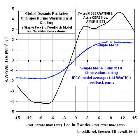
What we are REALLY interested in, though, is the optimum net feedback parameter for the model run. In this case, it was 1.25 Watts per sq. meter per deg. C. This corresponds to about 3 deg. C of warming for a doubling of atmospheric carbon dioxide (2XCO2, based upon an assumed radiative forcing of 3.7 Watts per sq. meter for 2XCO2). This is in approximate agreement with the IPCC’s best estimate for warming from 2XCO2, and supports the realism of the simple forcing-feedback model for determining climate sensitivity.

But note that the above simulation has 2 shortcomings: 1) it does not do a very good job of mimicking the warming up to 1940 and subsequent slight cooling to the 1970s; and (2) other than the major volcanic eruptions (e.g. Pinatubo in 1991), it does not mimic the sub-decadal temperature variations.

CASE #2: All GISS Forcings except Tropospheric Aerosols
Since the tropospheric aerosols have the largest uncertainty, it is instructive to see what the previous simulation would look like if we remove all 3 tropospheric aerosol components (aerosol reflection, black carbon, and aerosol indirect effect on clouds).

In that case an extremely similar fit to Case #1 is obtained, which has only a slightly degraded RMS error of 0.0788 deg. C.

This reveals that the addition of the tropospheric aerosols in the first run improved the model fit by only 3.2% compared to the run without tropospheric aerosols. Yet, what is particularly important is that the best fit feedback has now increased from 1.25 to 3.5 Watts per sq. meter per deg. C, which then reduces the 2XCO2 climate sensitivity from 3.0 deg. C to about 1.1 deg. C! This is below the 1.5 deg. C lower limit the IPCC has ‘very confidently” placed on that warming.

This illustrates the importance of assumed tropospheric aerosol pollution to the IPCC’s global warming arguments. Since the warming during the 20th Century was not as strong as would some expected from increasing greenhouse gases, an offsetting source of cooling had to be found – which, of course, was also manmade.

But even with those aerosols, the model fit to the observations was not very good. That’s where the PDO comes in.

CASE #3: PDO plus all GISS Forcings except Tropospheric Aerosols
For our third and final case, let’s see what happens when we replace the GISS tropospheric aerosol forcings – which are highly uncertain – with our satellite-inferred record of internal radiative forcing from the PDO.

The following plot shows that more of the previously unresolved temperature variability during the 20th Century is now captured; I have also included the “all GISS forcings” model fit for comparison:

Using the satellite observed PDO forcing of 0.6 Watts per sq. meter per unit change in the PDO index, the RMS error of the model fit improves by 25.4%, to 0.0588 deg. C; this can be compared to the much smaller 3.2% improvement from adding the GISS tropospheric aerosols.

If we ask what PDO-related forcing the model “prefers” to get a best fit, the satellite-inferred value of 0.6 is bumped up to around 1 Watt per sq. meter per unit change in the PDO index, with an RMS fit improvement of over 30% (not shown).

In this last model simulation, note the smaller temperature fluctuations in the HadCRUT3 surface temperature record are now better captured during the 20th Century. This is evidence that the PDO causes its own radiative forcing of the climate system.

And of particular interest, the substitution of the PDO forcing for the tropospheric aerosols restores the low climate sensitivity, with a preferred feedback parameter of 3.6, which corresponds to a 2XCO2 climate sensitivity of only 1.0 deg. C.

If you are wondering, including BOTH the GISS tropospheric aerosols and the PDO forcing made it difficult to get the model to come close to the observed temperature record. The best fit for this combination of forcings will have to wait till the full set of Monte Carlo computer simulations are made.

Conclusions

It is clear (to me, at least) that the IPCC’s claim that the sensitivity of the climate is quite high is critically dependent upon (1) the inclusion of very uncertain aerosol cooling effects in the last half of the 20th Century, and (2) the neglect of any sources of internal radiative forcing on long time scales, such as the 30-60 year time scale of the PDO.

Since we now have satellite measurements that such natural forcings do indeed exist, it would be advisable for the IPCC to revisit the issue of climate sensitivity, taking into account these uncertainties.

It would be difficult for the IPCC to fault this model because of its simplicity. For global average temperature changes on these time scales, the surface temperature variations are controlled by (1) radiative forcings, (2) net feedbacks, and (3) heat diffusion to the deeper ocean. In addition, the simple model’s assumption of a preferred average temperature is exactly what the IPCC implicitly claims! After all, they are the ones who say climate change did not occur until humans started polluting. Think hockey stick.

Remember, in the big picture, a given amount of global warming can be explained with either (1) weak forcing of a sensitive climate system, or (2) strong forcing of an insensitive climate system. By ignoring natural sources of warming – which are understandably less well known than anthropogenic sources — the IPCC biases its conclusions toward high climate sensitivity. I have addressed only ONE potential natural source of radiative forcing — the PDO. Of course, there could be others as well. But the 3rd Case presented above is already getting pretty close to the observed temperature record, which has its own uncertainties anyway.

This source of uncertainty — and bias — regarding the role of past, natural climate variations to the magnitude of future anthropogenic global warming (arghh! I mean climate change) is something that most climate scientists (let alone policymakers) do not yet understand.

WeatherShop.com Gifts, gadgets, weather stations, software and more...click here!

Evidence of Elevated Sea Surface Temperatures Under the BP Oil Slick

June 15th, 2010

(NOTE: minor edits made at 10:00 a.m. CDT, June 15, 2010)

As summer approaches, sea surface temperatures (SSTs) in the Gulf of Mexico increase in response to increased solar insolation (intensity of sunlight). Limiting the SST increase is evaporation, which increases nonlinearly with SST and approximately linearly with increased wind speed. It is important to realize that the primary heat loss mechanism by far for water bodies is evaporation.

By late summer, SSTs in the Gulf peak near 86 or 87 deg. F as these various energy gain and energy loss mechanisms approximately balance one another.

But yesterday, buoy 42040, moored about 64 nautical miles south of Dauphin Island, AL, reported a peak SST of 96 deg. F during very low wind conditions. Since the SST measurement is made about 1 meter below the sea surface, it is likely that even higher temperatures existed right at the surface…possibly in excess of 100 deg. F.

A nice global analysis of the day-night cycle in SSTs was published in 2003 by members of our NASA AMSR-E Science Team, which showed the normal range of this daytime warming, which increases at very low wind speed. But 96 deg. F is truly exceptional, especially for a measurement at 1 meter depth.

The following graph shows the last 45 days of SST measurements from this buoy, as well as buoy 42039 which is situated about 120 nautical miles to the east of buoy 42040.

The approximate locations of these buoys are shown in the following MODIS image from the Aqua satellite from 3 days ago (June 12, 2010); the oil slick areas are lighter colored patches, swirls and filaments, and can only be seen on days when the MODIS angle of view is near the point of sun glint (direct reflection of the sun’s image off the surface):

The day-night cycle in SSTs can be clearly seen on most days in the SST plot above, and it becomes stronger at lower wind speeds, as can be seen by comparing those SSTs to the measured wind speeds at these two buoys seen in the next plot:

Since buoy 42040 has been near the most persistent area of oil slick coverage seen by the MODIS instruments on NASA’s Terra and Aqua satellites, I think it is a fair supposition that these very high water temperatures are due to reduced evaporation from the oil film coverage on the sea surface.

OIL SLICK IMPACT ON GULF HURRICANES?
Despite the localized high SSTs, I do not believe that the oil slick will have an enhancement effect on the strength of hurricanes. The depth of water affected is probably pretty shallow, and restricted to areas with persistent oil sheen or slick that has not been disrupted by wind and wave activity.

As any hurricane approaches, higher winds will rapidly break up the oil on the surface, and mix the warmer surface layer with cooler, deeper layers. (Contrary to popular perception, the oil does not make the surface of the ocean darker and thereby absorb more sunlight…the ocean surface is already very dark and absorbs most of the sunlight that falls upon it — over 90%.)

Also, in order for any extra thermal energy to be available for a hurricane to use as fuel, it must be “converted” to more water vapor. Yes, hurricanes are on average strengthened over waters with higher SST, but only to the extent that the overlying atmosphere has its humidity enhanced by those higher SSTs. Evidence of reduced evaporation at buoy 42040 is seen in the following plot which shows the atmospheric temperature and dewpoint, as well as SST, for buoys 42040 (first plot), and 42039 (second plot).


Despite the elevated SSTs at buoy 42040 versus buoy 42039 in recent days, the dewpoint has not risen above what is being measured at buoy 42039 — if anything, it has remained lower.

Nevertheless, I suspect the issue of enhanced sea surface temperatures will be the subject of considerable future research, probably with computer modeling of the impact of such oil slicks on tropical cyclone intensity. I predict the effect will be very small.


Warming in Last 50 Years Predicted by Natural Climate Cycles

June 6th, 2010

One of the main conclusions of the 2007 IPCC report was that the warming over the last 50 years was most likely due to anthropogenic pollution, especially increasing atmospheric CO2 from fossil fuel burning.

But a minority of climate researchers have maintained that some — or even most — of that warming could have been due to natural causes. For instance, the Pacific Decadal Oscillation (PDO) and Atlantic Multi-decadal Oscillation (AMO) are natural modes of climate variability which have similar time scales to warming and cooling periods during the 20th Century. Also, El Nino — which is known to cause global-average warmth — has been more frequent in the last 30 years or so; the Southern Oscillation Index (SOI) is a measure of El Nino and La Nina activity.

A simple way to examine the possibility that these climate cycles might be involved in the warming over the last 50 years in to do a statistical comparison of the yearly temperature variations versus the PDO, AMO, and SOI yearly values. But of course, correlation does not prove causation.

So, what if we use the statistics BEFORE the last 50 years to come up with a model of temperature variability, and then see if that statistical model can “predict” the strong warming over the most recent 50 year period? That would be much more convincing because, if the relationship between temperature and these 3 climate indicies for the first half of the 20th Century just happened to be accidental, we sure wouldn’t expect it to accidentally predict the strong warming which has occurred in the second half of the 20th Century, would we?

Temperature, or Temperature Change Rate?
This kind of statistical comparison is usually performed with temperature. But there is greater physical justification for using the temperature change rate, instead of temperature. This is because if natural climate cycles are correlated to the time rate of change of temperature, that means they represent heating or cooling influences, such as changes in global cloud cover (albedo).

Such a relationship, shown in the plot below, would provide a causal link of these natural cycles as forcing mechanisms for temperature change, since the peak forcing then precedes the peak temperature.

Predicting Northern Hemispheric Warming Since 1960
Since most of the recent warming has occurred over the Northern Hemisphere, I chose to use the CRUTem3 yearly record of Northern Hemispheric temperature variations for the period 1900 through 2009. From this record I computed the yearly change rates in temperature. I then linearly regressed these 1-year temperature change rates against the yearly average values of the PDO, AMO, and SOI.

I used the period from 1900 through 1960 for “training” to derive this statistical relationship, then applied it to the period 1961 through 2009 to see how well it predicted the yearly temperature change rates for that 50 year period. Then, to get the model-predicted temperatures, I simply added up the temperature change rates over time.

The result of this exercise in shown in the following plot.

What is rather amazing is that the rate of observed warming of the Northern Hemisphere since the 1970’s matches that which the PDO, AMO, and SOI together predict, based upon those natural cycles’ PREVIOUS relationships to the temperature change rate (prior to 1960).

Again I want to emphasize that my use of the temperature change rate, rather than temperature, as the predicted variable is based upon the expectation that these natural modes of climate variability represent forcing mechanisms — I believe through changes in cloud cover — which then cause a lagged temperature response.

This is powerful evidence that most of the warming that the IPCC has attributed to human activities over the last 50 years could simply be due to natural, internal variability in the climate system. If true, this would also mean that (1) the climate system is much less sensitive to the CO2 content of the atmosphere than the IPCC claims, and (2) future warming from greenhouse gas emissions will be small.


Updated: Low Climate Sensitivity Estimated from the 11-Year Cycle in Total Solar Irradiance

June 4th, 2010

NOTE: This has been revised since finding an error in my analysis, so it replaces what was first published about an hour ago.

As part of an e-mail discussion on climate sensitivity I been having with a skeptic of my skepticism, he pointed me to a paper by Tung & Camp entitled Solar-Cycle Warming at the Earth’s Surface and an Observational Determination of Climate Sensitivity.

The authors try to determine just how much warming has occurred as a result of changing solar irradiance over the period 1959-2004. It appears that they use both the 11 year cycle, and a small increase in TSI over the period, as signals in their analysis. The paper purports to come up with a fairly high climate sensitivity that supports the IPCC’s estimated range, which then supports forecasts of substantial global warming from increasing greenhouse gas concentrations.

The authors start out in their first illustration with a straight comparison between yearly averages of TSI and global surface temperatures during 1959 through 2004. But rather than do a straightforward analysis of the average solar cycle to the average temperature cycle, the authors then go through a series of statistical acrobatics, focusing on those regions of the Earth which showed the greatest relationship between TSI variations and temperature.

I’m not sure, but I think this qualifies as cherry picking — only using those data that support your preconceived notion. They finally end up with a fairly high climate sensitivity, equivalent to about 3 deg. C of warming from a doubling of atmospheric CO2.

Tung and Camp claim their estimate is observationally based, free of any model assumptions. But this is wrong: they DO make assumptions based upon theory. For instance, it appears that they assume the temperature change is an equilibrium response to the forcing. Just because they used a calculator rather than a computer program to get their numbers does not mean their analysis is free of modeling assumptions.

But what bothers me the most is that there was a much simpler, and more defensible way to do the analysis than they presented.

A Simpler, More Physically-Based Analysis

The most obvious way I see to do such an analysis is to do a composite 11-year cycle in TSI (there were 4.5 solar cycles in their period of analysis, 1959 through 2004) and then compare it to a similarly composited 11-year cycle in surface temperatures. I took the TSI variations in their paper, and then used the HadCRUT3 global surface temperature anomalies. I detrended both time series first since it is the 11 year cycle which should be a robust solar signature…any long term temperature trends in the data could potentially be due to many things, and so it should not be included in such an analysis.

The following plot shows in the top panel my composited 11-year cycle in global average solar flux, after applying their correction for the surface area of the Earth (divide by 4), and correct for UV absorption by the stratosphere (multiply by 0.85). The bottom panel shows the corresponding 11-year cycle in global average surface temperatures. I have done a 3-year smoothing of the temperature data to help smooth out El Nino and La Nina related variations, which usually occur in adjacent years. I also took out the post-Pinatubo cooling years of 1992 and 1993, and interpolated back in values from the bounding years, 1991 and 1994.

Note there is a time lag of about 1 year between the solar forcing and the temperature response, as would be expected since it takes time for the upper ocean to warm.

It turns out this is a perfect opportunity to use the simple forcing-feedback model I have described before to see which value for the climate sensitivity provides the best fit to the observed temperature response to the 11-year cycle in solar forcing. The model can be expressed as:

Cp[dT/dt] = TSI – lambda*T,

Where Cp is the heat capacity of the climate system (dominated by the upper ocean), dT/dt is the change in temperature of the system with time, TSI represents the 11 year cycle in energy imbalance forcing of the system, and lambda*T is the net feedback upon temperature. It is the feedback parameter, lambda, that determines the climate sensitivity, so our goal is to find a value for a best value for lambda.

I ran the above model for a variety of ocean depths over which the heating/cooling is assumed to occur, and a variety of feedback parameters. The best fits between the observed and model-predicted temperature cycle (an example of which is shown in the lower panel of the above figure) occur for assumed ocean mixing depths around 25 meters, and a feedback parameter (lambda) of around 2.2 Watts per sq. meter per deg. C. Note the correlation of 0.97; the standard deviation of the difference between the modeled and observed temperature cycle is 0.012 deg. C

My best fit feedback (2.2 Watts per sq. meter per degree) produces a higher climate sensitivity (about 1.7 deg. C for a doubling of CO2) than what we have been finding from the satellite-derived feedback, which runs around 6 Watts per sq. meter per degree (corresponding to about 0.55 deg. C of warming).

Can High Climate Sensitivity Explain the Data, Too?

If I instead run the model with the lambda value Tung and Camp get (1.25), the modeled temperature exhibits too much time lag between the solar forcing and temperature response….about double that produced with a feedback of 2.2.

Discussion

The results of this experiment are pretty sensitive to errors in the observed temperatures, since we are talking about the response to a very small forcing — less than 0.2 Watts per sq. meter from solar max to solar min. This is an extremely small forcing to expect a robust global-average temperature response from.

If someone else has published an analysis similar to what I have just presented, please let me know…I find it hard to believe someone has not done this before. I would be nice if someone else went through the same exercise and got the same answers. Similarly, let me know if you think I have made an error.

I think the methodology I have presented is the most physically-based and easiest way to estimate climate sensitivity from the 11-year cycle in solar flux averaged over the Earth, and the resulting 11-year cycle in global surface temperatures. It conserves energy, and makes no assumptions about the temperature being in equilibrium with the forcing.

I have ignored the possibility of any Svensmark-type mechanism of cloud modulation by the solar cycle…this will have to remain a source of uncertainty for now.

The bottom line is that my analysis supports a best-estimate 2XCO2 climate sensitivity of 1.7 deg. C, which is little more than half of that obtained by Tung & Camp (3.0 deg. C), and approaches the lower limit of what the IPCC claims is likely (1.5 deg. C).