UAH Global Temperature Update for August 2020: +0.43 deg. C

September 1st, 2020

The Version 6.0 global average lower tropospheric temperature (LT) anomaly for August, 2020 was +0.43 deg. C, essentially unchanged from the July, 2020 value of +0.44 deg. C.

The linear warming trend since January, 1979 remains at +0.14 C/decade (+0.12 C/decade over the global-averaged oceans, and +0.18 C/decade over global-averaged land).

Various regional LT departures from the 30-year (1981-2010) average for the last 20 months are:

 YEAR MO GLOBE NHEM. SHEM. TROPIC USA48 ARCTIC AUST 
2019 01 +0.38 +0.35 +0.41 +0.35 +0.53 -0.14 +1.14
2019 02 +0.37 +0.47 +0.28 +0.43 -0.02 +1.05 +0.05
2019 03 +0.34 +0.44 +0.25 +0.41 -0.55 +0.97 +0.58
2019 04 +0.44 +0.38 +0.51 +0.53 +0.49 +0.93 +0.91
2019 05 +0.32 +0.29 +0.35 +0.39 -0.61 +0.99 +0.38
2019 06 +0.47 +0.42 +0.52 +0.64 -0.64 +0.91 +0.35
2019 07 +0.38 +0.33 +0.44 +0.45 +0.10 +0.34 +0.87
2019 08 +0.38 +0.38 +0.39 +0.42 +0.17 +0.44 +0.23
2019 09 +0.61 +0.64 +0.59 +0.60 +1.14 +0.75 +0.57
2019 10 +0.46 +0.64 +0.27 +0.30 -0.03 +1.00 +0.49
2019 11 +0.55 +0.56 +0.54 +0.55 +0.21 +0.56 +0.37
2019 12 +0.56 +0.61 +0.50 +0.58 +0.92 +0.66 +0.94
2020 01 +0.56 +0.60 +0.53 +0.61 +0.73 +0.12 +0.65
2020 02 +0.75 +0.96 +0.55 +0.76 +0.38 +0.02 +0.30
2020 03 +0.47 +0.61 +0.34 +0.63 +1.09 -0.72 +0.16
2020 04 +0.38 +0.43 +0.33 +0.45 -0.59 +1.03 +0.97
2020 05 +0.54 +0.60 +0.49 +0.66 +0.17 +1.16 -0.15
2020 06 +0.43 +0.45 +0.41 +0.46 +0.38 +0.80 +1.20
2020 07 +0.44 +0.45 +0.42 +0.46 +0.56 +0.40 +0.66
2020 08 +0.43 +0.47 +0.38 +0.59 +0.41 +0.47 +0.49

The full UAH Global Temperature Report, along with the LT global gridpoint anomaly image for August, 2020 should be available within the next few days here.

The global and regional monthly anomalies for the various atmospheric layers we monitor should be available in the next few days at the following locations:

Lower Troposphere: http://vortex.nsstc.uah.edu/data/msu/v6.0/tlt/uahncdc_lt_6.0.txt
Mid-Troposphere: http://vortex.nsstc.uah.edu/data/msu/v6.0/tmt/uahncdc_mt_6.0.txt
Tropopause: http://vortex.nsstc.uah.edu/data/msu/v6.0/ttp/uahncdc_tp_6.0.txt
Lower Stratosphere: http://vortex.nsstc.uah.edu/data/msu/v6.0/tls/uahncdc_ls_6.0.txt

Even with Laura, Louisiana Hurricanes Have Not Increased Since 1851

August 26th, 2020

As I write this, it looks like major Hurricane Laura will arrive on the Louisiana coast late tonight as a Category 4 hurricane somewhere south of Lake Charles.

Fig. 1. GOES-East Geocolor image of major Hurricane Laura heading toward the southwest Louisiana coast at 9:50 a.m. CDT 26 August 2020.

There will be the inevitable fake news coverage claiming how U.S. landfalling hurricanes are getting worse, a subject which I addressed in my Amazon Kindle e-book Inevitable Disaster: Why Hurricanes Can’t Be Blamed on Global Warming.

Of course, hurricane damage has increased, as people flock to the nation’s coasts and associated infrastructure increases. But we should remember that (for example) Miami only had 444 residents when incorporated in 1896, and now the Miami metroplex has over 6,000,000 inhabitants.

So, yes, storm damage will increase, but not because the weather has gotten worse.

Given the current event, which is sure to bring major damage to southwest Louisiana, I thought I would present the statistics for all documented hurricanes affecting Louisiana in the last 170 years (1851-2020).

Neither Hurricane Numbers nor Intensities Have Increased in Louisiana

If we examine all of the hurricanes affecting Louisiana in the last 170 years in the National Hurricane Center’s HURDAT database (as summarized on Wikipedia) we find that there has been no long-term increase in either the number of hurricanes or their intensity since 1851.

Fig. 2. Neither the number nor intensity of hurricanes impacting Louisiana since 1851 have experienced a long-term increase, assuming major Hurricane Laura (2020) makes landfall as a Cat4 storm. Dashed lines are the linear trends.

Again, this is based upon official NOAA National Hurricane Center (NHC) statistics.

UAH Global Temperature Update for July 2020: +0.44 deg. C

August 3rd, 2020

The Version 6.0 global average lower tropospheric temperature (LT) anomaly for July, 2020 was +0.44 deg. C, essentially unchanged from the June, 2020 value of +0.43 deg. C.

The linear warming trend since January, 1979 remains at +0.14 C/decade (+0.12 C/decade over the global-averaged oceans, and +0.18 C/decade over global-averaged land).

Various regional LT departures from the 30-year (1981-2010) average for the last 19 months are:

 YEAR MO GLOBE NHEM. SHEM. TROPIC USA48 ARCTIC AUST 
2019 01 +0.38 +0.35 +0.41 +0.36 +0.53 -0.14 +1.14
2019 02 +0.37 +0.47 +0.28 +0.43 -0.02 +1.05 +0.05
2019 03 +0.34 +0.44 +0.25 +0.41 -0.55 +0.97 +0.58
2019 04 +0.44 +0.38 +0.51 +0.54 +0.50 +0.93 +0.91
2019 05 +0.32 +0.29 +0.35 +0.39 -0.61 +0.99 +0.38
2019 06 +0.47 +0.42 +0.52 +0.64 -0.64 +0.91 +0.35
2019 07 +0.38 +0.33 +0.44 +0.45 +0.11 +0.34 +0.87
2019 08 +0.39 +0.38 +0.39 +0.42 +0.17 +0.44 +0.23
2019 09 +0.61 +0.64 +0.59 +0.60 +1.14 +0.75 +0.57
2019 10 +0.46 +0.64 +0.27 +0.30 -0.03 +1.00 +0.49
2019 11 +0.55 +0.56 +0.54 +0.55 +0.21 +0.56 +0.37
2019 12 +0.56 +0.61 +0.50 +0.58 +0.92 +0.66 +0.94
2020 01 +0.56 +0.60 +0.53 +0.61 +0.73 +0.13 +0.65
2020 02 +0.76 +0.96 +0.55 +0.76 +0.38 +0.02 +0.30
2020 03 +0.48 +0.61 +0.34 +0.63 +1.09 -0.72 +0.16
2020 04 +0.38 +0.43 +0.33 +0.45 -0.59 +1.03 +0.97
2020 05 +0.54 +0.60 +0.49 +0.66 +0.17 +1.16 -0.15
2020 06 +0.43 +0.45 +0.41 +0.46 +0.38 +0.80 +1.20
2020 07 +0.44 +0.45 +0.42 +0.46 +0.56 +0.40 +0.66

The full UAH Global Temperature Report, along with the LT global gridpoint anomaly image for July, 2020 should be available within the next few days here.

The global and regional monthly anomalies for the various atmospheric layers we monitor should be available in the next few days at the following locations:

Lower Troposphere: http://vortex.nsstc.uah.edu/data/msu/v6.0/tlt/uahncdc_lt_6.0.txt
Mid-Troposphere: http://vortex.nsstc.uah.edu/data/msu/v6.0/tmt/uahncdc_mt_6.0.txt
Tropopause: http://vortex.nsstc.uah.edu/data/msu/v6.0/ttp/uahncdc_tp_6.0.txt
Lower Stratosphere: http://vortex.nsstc.uah.edu/data/msu/v6.0/tls/uahncdc_ls_6.0.txt

Time Lapse Video of Altocumulus with Virga

July 14th, 2020

I’ve always wanted to capture this kind of cloud as a time lapse. I noticed them on my way to work this morning, and had a camera and tripod with me, so this was my chance.

These are altocumulus clouds with strong upward motion in them producing precipitation, in this case snow, falling in streaks and not reaching the ground (“virga”). They form when the upper troposphere is unstable, and warm advection (a warm air mass moving into a cool air mass) produces the uplift.

Lightning strike video close-up

July 13th, 2020

We live next to a 1,500 ft tall TV tower which frequently gets hit by lightning. We are so close, in fact, that it is difficult to get good photographs because the area just above the tower top is at an elevation angle of 70 deg. viewed from our yard, which is too steep to take pictures through a window, and for outdoor photos will cause rain to fall on the camera lens.

So, despite thousands of lightning strikes we have witnessed and heard over the years, I seldom attempt photos or video. Yesterday was one of the rare instances where the thunderstorm anvil trailing downwind of the approaching storm was sending out lightning strokes at regular, ~2 minute intervals before the rain began. This is the best time to watch the lightning for us, usually by lying down on an outdoor lounge chair and looking almost straight up.

My camera equipment was still in the car from a short trip to take photos of Comet NEOWISE the previous morning. Sensing this was a chance to capture some good video, I ran out to the car, retrieved my camera backpack and a tripod, and ran to the backyard. I set up the camera and tripod in record time, quickly adjusted the focus manually, and hit the record button.

In literally less than 1 second after pressing the record button, the best strike of the storm occurred. Here’s an animated GIF of the event… 20 video frame captures at 1/24 sec intervals (the vertical scale is exaggerated because I forced WordPress to load the full-resolution file… click on the video to see the proper perspective):

There are a lot of interesting features that I won’t go into here, except I especially like how the ionized channel breaks up into pockets of glowing air during dissipation, here’s one of the frames showing that structure:

Observed Decrease in U.S. Child Mortality During the COVID-19 Lockdown of 2020

July 10th, 2020

Overview: Death certificate data, corrected for recent under-reporting, reveals a 10-20% decrease in weekly deaths compared to seasonal norms commencing in early March, 2020. This date coincides with the widespread closing of public schools. It is hypothesized that a decrease in traffic accidents is the most likely explanation for the decrease, a conclusion which would be confirmed from detailed analysis of the death certificate data.

I had previously blogged on the caution needed when analyzing the death counts from death certificate data compiled by the CDC. The most recent weeks always have under-counted totals because it takes weeks to months for all of the death certificates to trickle in and be counted. Use of the data without knowing this can lead to false conclusions about recently declining death rates. I outlined a simple method for doing a first-order correction of the data based upon the number of additional death reports in each successive week, a method which I use here.

The CDC data report weekly deaths in three age groups: less than 18 years old (“child”), 18-64, and 65 on up. The data are updated weekly, and the data online extend back to week 40 in 2015. I examined the death totals for the under-18 year old group versus the totals for the 18-and-older (combined) group. (Only those recent reports that were labeled as “100% reporting” were used, but this notation is misleading because the CDC means 100% of the locations around the country had submitted reports, not that all of the reports were complete.)

I removed the average seasonal cycle (2016-2019) from the weekly totals, which show a seasonal ~11% peak in deaths in early January for adults, and a weaker ~6% peak in children’s deaths in early June (Fig. 1).

Fig. 1. Seasonal variations (%) in deaths (all causes) for adults versus children, 2016 through 2019.

In order to corrected for under-reporting of recent deaths, I used the data from 4 successive weeks earlier this year to correct the most recent 52 weeks of data. Those 4 successive weeks yielded average week-to-week adjustments which accumulated to 16.5% under-reporting for 1 week previous to latest reported week; 10.4% at 2 weeks previous; 7.8% at 3 weeks; 6.4% at 4 weeks, dropping below 1% at 10 weeks previous, etc.

I then computed the weekly percent departures from the average seasonal cycle for the entire time period (since week 40 of 2015). The results (Fig. 2) show the unusually bad peak in seasonal flu and pneumonia deaths in 2017-18, which as expected results in a larger increase in adults that children.

Fig. 2. Weekly number of deaths as percent departures from seasonal normals, for adults versus children, plotted as a phase space diagram (successive weeks connected by a line).

Note that there is a 10-20% decrease in child deaths beginning in early March, which is when most schools in the U.S closed down. Since the most frequent cause of death in the under-18 age group is auto accidents, it makes sense that the greatly reduced traffic activity during “lockdown” led to fewer deaths.

Of course, the same kind of reduction would be expected in the adult age category, but it is completely overwhelmed in Fig. 2 by the large increase due to COVID-19 deaths, which peaked in mid-April. Since there have been very few COVID-19 deaths in children we more clearly see the reduction in that age group. In absolute terms, a 15% reduction in childhood deaths equates to about 85 children per week. 

Hot Summer Epic Fail: New Climate Models Exaggerate Midwest Warming by 6X

July 3rd, 2020

For the last 10 years I have consulted for grain growing interests, providing information about past and potential future trends in growing season weather that might impact crop yields. Their primary interest is the U.S. corn belt, particularly the 12 Midwest states (Iowa, Illinois, Indiana, Ohio, Kansas, Nebraska, Missouri, Oklahoma, the Dakotas, Minnesota, and Michigan) which produce most of the U.S. corn and soybean crop.

Contrary to popular perception, the U.S. Midwest has seen little long-term summer warming. For precipitation, the slight drying predicted by climate models in response to human greenhouse gas emissions has not occurred; if anything, precipitation has increased. Corn yield trends continue on a technologically-driven upward trajectory, totally obscuring any potential negative impact of “climate change”.

What Period of Time Should We Examine to Test Global Warming Claims?

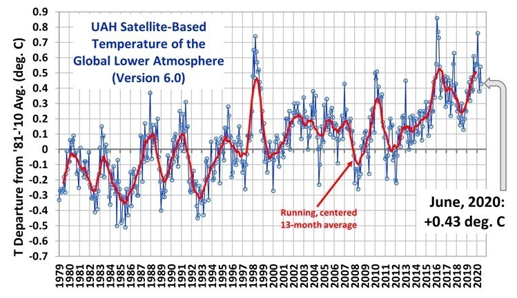
Based upon the observations, “global warming” did not really begin until the late 1970s. Prior to that time, anthropogenic greenhouse gas emissions had not yet increased by much at all, and natural climate variability dominated the observational record (and some say it still does).

Furthermore, uncertainties regarding the cooling effects of sulfate aerosol pollution make any model predictions before the 1970s-80s suspect since modelers simply adjusted the aerosol cooling effect in their models to match the temperature observations, which showed little if any warming before that time which could be reasonably attributed to greenhouse gas emissions.

This is why I am emphasizing the last 50 years (1970-2019)…this is the period during which we should have seen the strongest warming, and as greenhouse gas emissions continue to increase, it is the period of most interest to help determine just how much faith we should put into model predictions for changes in national energy policies. In other words, quantitative testing of greenhouse warming theory should be during a period when the signal of that warming is expected to be the greatest.

50 Years of Predictions vs. Observations

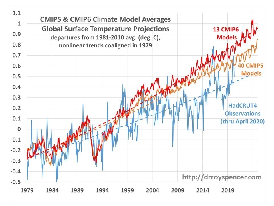
Now that the new CMIP6 climate model experiment data are becoming available, we can begin to get some idea of how those models are shaping up against observations and the previous (CMIP5) model predictions. The following analysis includes the available model out put at the KNMI Climate Explorer website. The temperature observations come from the statewide data at NOAA’s Climate at a Glance website.

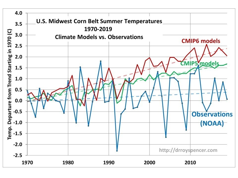
For the Midwest U.S. in the summer (June-July-August) we see that there has been almost no statistically significant warming in the last 50 years, whereas the CMIP6 models appear to be producing even more warming than the CMIP5 models did.

Fifty years (1970-2019) of U.S. corn belt summer (JJA) warming since 1970 from observations (blue); the previous CMIP5 climate models (42 model avg., green); and the new CMIP6 climate models (13 model avg., red). The three time series have been vertically aligned so their trend lines coincide in the first year (1970), which is the most meaningful way to quantify the long-term warming since 1970.

The observed 50-year trend is only 0.086 C/decade (barely significant at the 1-sigma level), while the CMIP5 average model trend is 4X as large at 0.343 C/decade, and the CMIP6 trend is 5.7X as large at 0.495 C/decade. While the CMIP6 trend will change somewhat as more models are added, it is consistent with the report that the CMIP6 models are producing more average warming than their CMIP5 predecessors.

I am showing the average of the available models rather than individual models, because it is the average of the models which guides the UN IPCC reports and thus energy policy. It is disingenuous for some to claim that “not all IPCC models disagree with the observations”, as if that is some sort of vindication of all the models. It is not. If there are one or two models that agree the best with observations, why isn’t the IPCC just using those to write its reports? Hmmm?

What I find particularly troubling is that the climate modelers are increasingly deaf to what observations tell us. How can the CMIP5 models (let alone the newer CMIP6 models) be used to guide U.S. energy policy when there is such a huge discrepancy between the models and the observations?

I realize this is just one season (summer) in one region (the U.S. Midwest), but it is immensely important. The U.S. is the world leader in production of corn (which is used for feed, food, and fuel) and behind only Brazil in soybean production. Blatantly false claims (e.g. here) of observed change in Midwest climate have fed the popular opinion that U.S. crops are already feeling the negative effects of human-caused climate change, despite the facts.

This is just one example of many that the news media have been complicit in the destruction of rational climate debate, which is now extending to outright censoring of alternative climate views on not only social media, but also in mainstream news sources like Forbes which disappeared environmentalist Michael Shellenberger’s op-ed in which he confessed he no longer believes in a “climate crisis”.

UAH Global Temperature Update for June 2020: +0.43 deg. C

July 2nd, 2020

The Version 6.0 global average lower tropospheric temperature (LT) anomaly for June, 2020 was +0.43 deg. C, down from the May, 2020 value of +0.54 deg. C.

The linear warming trend since January, 1979 is +0.14 C/decade (+0.12 C/decade over the global-averaged oceans, and +0.18 C/decade over global-averaged land).

Various regional LT departures from the 30-year (1981-2010) average for the last 18 months are:

 YEAR MO GLOBE NHEM. SHEM. TROPIC USA48 ARCTIC AUST 
2019 01 +0.38 +0.35 +0.41 +0.36 +0.53 -0.14 +1.15
2019 02 +0.37 +0.47 +0.28 +0.43 -0.02 +1.05 +0.05
2019 03 +0.34 +0.44 +0.25 +0.41 -0.55 +0.97 +0.58
2019 04 +0.44 +0.38 +0.51 +0.54 +0.49 +0.93 +0.91
2019 05 +0.32 +0.29 +0.35 +0.39 -0.61 +0.99 +0.38
2019 06 +0.47 +0.42 +0.52 +0.64 -0.64 +0.91 +0.35
2019 07 +0.38 +0.33 +0.44 +0.45 +0.11 +0.34 +0.87
2019 08 +0.39 +0.38 +0.39 +0.42 +0.17 +0.44 +0.23
2019 09 +0.61 +0.64 +0.59 +0.60 +1.14 +0.75 +0.57
2019 10 +0.46 +0.64 +0.27 +0.30 -0.03 +1.00 +0.49
2019 11 +0.55 +0.56 +0.54 +0.55 +0.21 +0.56 +0.38
2019 12 +0.56 +0.61 +0.50 +0.58 +0.92 +0.66 +0.94
2020 01 +0.56 +0.60 +0.53 +0.61 +0.73 +0.12 +0.66
2020 02 +0.76 +0.96 +0.55 +0.76 +0.38 +0.02 +0.30
2020 03 +0.48 +0.61 +0.34 +0.63 +1.09 -0.72 +0.16
2020 04 +0.38 +0.43 +0.34 +0.45 -0.59 +1.03 +0.97
2020 05 +0.54 +0.60 +0.49 +0.66 +0.17 +1.15 -0.15
2020 06 +0.43 +0.45 +0.41 +0.46 +0.38 +0.80 +1.20

The UAH LT global gridpoint anomaly image for June, 2020 should be available within the next week here.

The global and regional monthly anomalies for the various atmospheric layers we monitor should be available in the next few days at the following locations:

Lower Troposphere: http://vortex.nsstc.uah.edu/data/msu/v6.0/tlt/uahncdc_lt_6.0.txt
Mid-Troposphere: http://vortex.nsstc.uah.edu/data/msu/v6.0/tmt/uahncdc_mt_6.0.txt
Tropopause: http://vortex.nsstc.uah.edu/data/msu/v6.0/ttp/uahncdc_tp_6.0.txt
Lower Stratosphere: http://vortex.nsstc.uah.edu/data/msu/v6.0/tls/uahncdc_ls_6.0.txt

CMIP6 Climate Models Producing 50% More Surface Warming than Observations since 1979

June 25th, 2020

Those who defend climate model predictions often produce plots of observed surface temperature compared to the models which show very good agreement. Setting aside the debate over the continuing adjustments to the surface temperature record which produce ever-increasing warming trends, let’s look at how the most recent (CMIP6) models are doing compared to the latest version of the observations (however good those are).

First, I’d like to explain how some authors get such good agreement between the models and observations. Here are the two “techniques” they use that most annoy me.

  1. They look at long periods of time, say the last 100+ years. This improves the apparent agreement because most of that period was before there was substantial forcing of the climate system by increasing CO2.
  2. They plot anomalies about a common reference period, but do not show trend lines. Or, if they show trends lines, they do not start them at the same point at the beginning of the record. When you do this, the discrepancy between models and observations is split in half, with the discrepancy in the latter half of the record having the opposite sign of the discrepancy in the early part of the record. They say, “See? The observed temperatures in the last few decades nearly match the models!”

In the following plot (which will be included in a report I am doing for the Global Warming Policy Foundation) I avoid both of those problems. During the period of strongest greenhouse gas forcing (since 1979), the latest CMIP6 models reveal 50% more net surface warming from 1979 up to April 2020 (+1.08 deg. C) than do the observations (+0.72 deg. C).

Note I have accounted for the trends being somewhat nonlinear, using a 2nd order polynomial fit to all three time series. Next, I have adjusted the CMIP time series vertically so that their polynomial fit lines are coaligned with the observations in 1979. I believe this is the most honest and meaningful way to intercompare the warming trends in different datasets.

As others have noted, it appears the CMIP6 models are producing even more warming than the CMIP5 models did… although the KNMI Climate Explorer website (from which all of the data was downloaded) has only 13 models archived so far.

COVID-19 Global Economic Downturn not Affecting CO2 Rise: May 2020 Update

June 5th, 2020

The Mauna Loa atmospheric CO2 concentration data continue to show no reduction in the rate of rise due to the recent global economic slowdown. This demonstrates how difficult it is to reduce global CO2 emissions without causing a major disruption to the global economy and exacerbation of poverty.

After removal of the strong seasonal cycle in Mauna Loa CO2 data, and a first order estimate of the CO2 influence of El Nino and La Nina activity (ENSO), the May 2020 update shows no indication of a reduction in the rate of rise in the last few months, when the reduction in economic activity should have shown up.

I had previously explained why the slowdown would likely not be large enough to affect measured atmospheric CO2 levels compared to natural variations in global sources and sinks of CO2. I calculated that the Energy Information Administration-estimated 11% reductions in CO2 emissions during 2020 would have to be four times larger to stop the rise of atmospheric CO2 over 2019 values (assuming no substantial natural variations in CO2 sources and sinks).