I’ve received many more requests about the new disappearing-clouds study than the “gold standard proof of anthropogenic warming” study I addressed here, both of which appeared in Nature journals over the last several days.
The widespread interest is partly because of the way the study is dramatized in the media. For example, check out this headline, “A World Without Clouds“, and the study’s forecast of 12 deg. C of global warming.
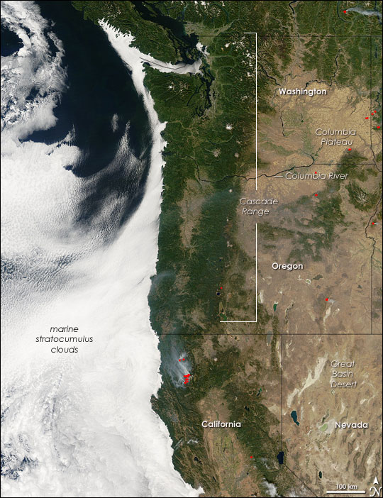
The disappearing clouds study is based upon the modelling of marine stratocumulus clouds, whose existence substantially cools the Earth. These extensive but shallow cloud decks cover the subtropical ocean regions over the eastern ocean basins where upwelling cold water creates a strong boundary layer inversion.
Marine stratocumulus clouds off the U.S. West Coast, which form in a water-chilled shallow layer of boundary layer air capped by warmer air aloft (NASA/GSFC).
In other words, the cold water causes a thin marine boundary layer of chilled air up to a kilometer deep, than is capped by warmer air aloft. The resulting inversion layer (the boundary between cool air below and warm air aloft) inhibits convective mixing, and so water evaporated from the ocean accumulates in the boundary layer and clouds then develop at the base of the inversion. There are complex infrared radiative processes which also help maintain the cloud layer.
The new modeling study describes how these cloud layers could dissipate if atmospheric CO2 concentrations get too high, thus causing a positive feedback loop on warming and greatly increasing future global temperatures, even beyond what the IPCC has predicted from global climate models. The marine stratocumulus cloud response to warming is not a new issue, as modelers have been debating for decades whether these clouds would increase or decrease with warming, thus either reducing or amplifying the small amount of direct radiative warming from increasing CO2.
The new study uses a very high resolution model that “grows” the marine stratocumulus clouds. The IPCC’s climate models, in contrast, have much lower resolution and must parameterize the existence of the clouds based upon larger-scale model variables. These high resolution models have been around for many years, but this study tries to specifically address how increasing CO2 in the whole atmosphere changes this thin, but important, cloud layer.
The high resolution simulations are stunning in their realism, covering a domain of 4.8 x 4.8 km:
The main conclusion of the study is that when model CO2 concentrations reach 1200 ppm or so (which would take as little as another 100 years or so assuming worst-case energy use and population growth projections like RCP8.5), a substantial dissipation of these clouds occurs causing substantial additional global warming, with up to 12 deg. C of total global warming.
Shortcomings in the Study: The Large-Scale Ocean and Atmospheric Environment
All studies like this require assumptions. In my view, the problem is not with the high-resolution model of the clouds itself. Instead, it’s the assumed state of the large-scale environment in which the clouds are assumed to be embedded.
Most importantly, it should be remembered that these clouds exist where cold water is upwelling from the deep ocean, where it has resided for centuries to millennia after initially being chilled to near-freezing in polar regions, and flowing in from higher latitudes. This cold water is continually feeding the stratocumulus zones, helping to maintain the strong temperature inversion at the top of the chilled marine boundary layer. Instead, their model has 1 meter thick slab ocean that rapidly responds to only whats going on with atmospheric greenhouse gases within the tiny (5 km) model domain. Such a shallow ocean layer would be ok (as they claim) IF the ocean portion of the model was a closed system… the shallow ocean only increases how rapidly the model responds… not its final equilibrium state. But given the continuous influx of cold water into these stratocumulus regions from below and from high latitudes in nature, it is far from a closed system.
Second, the atmospheric environment in which the high-res cloud model is embedded is assumed to have similar characteristics to what climate models produce. This includes substantial increases in free-tropospheric water vapor, keeping constant relative humidity throughout the troposphere. In climate models, the enhanced infrared effects of this absolute increase in water vapor leads to a tropical “hot spot”, which observations, so far, fail to show. This is a second reason the study’s results are exaggerated. Part of the disappearing cloud effect in their model is from increased downwelling radiation from the free troposphere as CO2 increases and positive water vapor feedback in the global climate models increases downwelling IR even more. This reduces the rate of infrared cooling by the cloud tops, which is one process that normally maintains them. The model clouds then disappear, causing more sunlight to flood in and warm the isolated shallow slab ocean. But if the free troposphere above the cloud does not produce nearly as large an effect from increasing water vapor, the clouds will not show such a dramatic effect.
The bottom line is that marine stratocumulus clouds exist because of the strong temperature inversion maintained by cold water from upwelling and transport from high latitudes. That chilled boundary layer air bumps up against warm free-tropospheric air (warmed, in turn, by subsidence forced by moist air ascent in precipitation systems possibly thousands of miles away). That inversion will likely be well-maintained in a warming world, thus maintaining the cloud deck, and not causing catastrophic global warming.
A new paper in Nature Climate Change by Santer et al. (paywalled) claims that the 40 year record of global tropospheric temperatures agrees with climate model simulations of anthropogenic global warming so well that there is less than a 1 in 3.5 million chance (5 sigma, one-tailed test) that the agreement between models and satellites is just by chance.
And, yes, that applies to our (UAH) dataset as well.
While it’s nice that the authors commemorate 40 years of satellite temperature monitoring method (which John Christy and I originally developed), I’m dismayed that this published result could feed a new “one in a million” meme that rivals the “97% of scientists agree” meme, which has been a very successful talking point for politicians, journalists, and liberal arts majors.
John Christy and I examined the study to see just what was done. I will give you the bottom line first, in case you don’t have time to wade through the details:
The new Santer et al. study merely shows that the satellite data have indeed detected warming (not saying how much) that the models can currently only explain with increasing CO2 (since they cannot yet reproduce natural climate variability on multi-decadal time scales).
That’s all.
But we already knew that, didn’t we? So why publish a paper that goes to such great lengths to demonstrate it with an absurdly exaggerated statistic such as 1 in 3.5 million (which corresponds to 99.99997% confidence)? I’ll leave that as a rhetorical question for you to ponder.T
There is so much that should be said, it’s hard to know where to begin.
Current climate models are programmed to only produce human-caused warming
First, you must realize that ANY source of temperature change in the climate system, whether externally forced (e.g. increasing CO2, volcanoes) or internally forced (e.g. weakening ocean vertical circulation, stronger El Ninos) has about the same global temperature signature regionally: more change over land than ocean (yes, even if the ocean is the original source of warming), and as a consequence more warming over the Northern than Southern Hemisphere. In addition, the models tend to warm the tropics more than the extratropics, a pattern which the satellite measurements do not particularly agree with.
Current climate model are adjusted in a rather ad hoc manner to produce no long-term warming (or cooling). This is because the global radiative energy balance that maintains temperatures at a relatively constant level is not known accurately enough from first physical principles (or even from observations), so any unforced trends in the models are considered “spurious” and removed. A handful of weak time-dependent forcings (e.g. ozone depletion, aerosol cooling) are then included in the models which can nudge them somewhat in the warmer or cooler direction temporarily, but only increasing CO2 can cause substantial model warming.
Importantly, we don’t understand natural climate variations, and the models don’t produce it, so CO2 is the only source of warming in today’s state-of-the-art models.
The New Study Methodology
The Santer et al. study address the 40-year period (1979-2018) of tropospheric temperature measurements. They average the models regional pattern of warming during that time, and see how well the satellite data match the models for the geographic pattern.
A few points must be made about this methodology.
As previously mentioned, the models already assume that only CO2 can produce warming, and so their finding of some agreement between model warming and satellite-observed warming is taken to mean proof that the warming is human-caused. It is not. Any natural source of warming (as we will see) would produce about the same kind of agreement, but the models have already been adjusted to exclude that possibility.
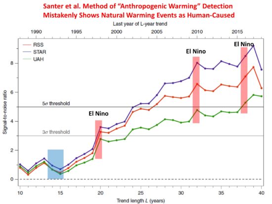
Proof of point #1 can be seen in their plot (below) of how the agreement between models and satellite observations increases over time. The fact that the agreement surges during major El Nino warm events is evidence that natural sources of warming can be mis-diagnosed as an anthropogenic signature. What if there is also a multi-decadal source of warming, as has been found to be missing in models compared to observations (e.g. Kravtsov et al., 2018)?
John Christy pointed out that the two major volcanic eruptions (El Chichon and Pinatubo, the latter shown as a blue box in the plot below), which caused temporary cooling, were in the early part of the 40 year record. Even if the model runs did not include increasing CO2, there would still be agreement between warming trends in the models and observations just because of the volcanic cooling early would lead to positive 40-year trends. Obviously, this agreement would not indicate an anthropogenic source, even though the authors methodology would identify it as such.
Their metric for measuring agreement between models and observations basically multiplies the regional warming pattern in the models with the regional warming pattern in the observations. If these patterns were totally uncorrelated, then there would be no diagnosed agreement. But this tells us little about the MAGNITUDE of warming in the observations agreeing with the models. The warming in the observations might only be 1/3 that of the models, or alternatively the warming in the models might be only 1/3 that in the observations. Their metric gives the same value either way. All that is necessary is for the temperature change to be of the same sign, and more warming in either the models or observations will cause an diagnosed increase in the level of agreement metric they use, even if the warming trends are diverging over time.
Their metric of agreement does not even need a geographic “pattern” of warming to reach an absurdly high level of statistical agreement. Warming could be the same everywhere in their 576 gridpoints covering most the Earth, and their metric would sum up the agreement at every gridpoint as independent evidence of a “pattern agreement”, even though no “pattern” of warming exists. This seems like a rather exaggerated statistic.
These are just some of my first impressions of the new study. Ross McKitrick is also examining the paper and will probably have a more elegant explanation of the statistics the paper uses and what those statistics can and cannot show.
Nevertheless, the metric used does demonstrate some level of agreement with high confidence. What exactly is it? As far as I can tell, it’s simply that the satellite observations show some warming in the last 40 years, and so do the models. The expected pattern is fairly uniform globally, which does not tell us much since even El Nino produces fairly uniform warming (and volcanoes produce global cooling). Yet their statistic seems to treat each of the 576 gridpoints as independent, which should have been taken into account (similar to time autocorrelation in time series). It will take more time to examine whether this is indeed the case.
In the end, I believe the study is an attempt to exaggerate the level of agreement between satellite (even UAH) and model warming trends, providing supposed “proof” that the warming is due to increasing CO2, even though natural sources of temperature change (temporary El Nino warming, volcanic cooling early in the record, and who knows what else) can be misinterpreted by their method as human-caused warming.
There is no shortage of articles claiming that global warming is causing agriculture of certain crops to push farther north, for example into the southern Canadian Prairie provinces of Manitoba and Saskatchewan.
My contacts in the grain trading business tell me that the belief is widespread.
For example, here’s a quote from a Manitoba Co-operator article,
Lutz Goedde, of the management and consulting firm McKinsey & Company, said Canada is in a unique position because of its northern latitude and large supply of fresh water…. Pointing to the steady northward trek of corn and soybeans, the agricultural business consultant said that the effects are already evident.
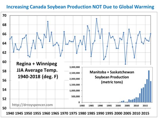
The problem with this view is that the two main weather stations located in this region (Regina and Winnipeg) do not show a statistically significant warming trend during the prime growing months of June, July, and August:
Average yearly growing season temperatures at Regina and Winnipeg show no obvious warming trend that might explain the rapid increase in soybean production in southern Manitoba and Saskatchewan since 2000. Temperature data from Environment and Climate Change Canada.
So what is really happening? The amount of various grains produced each year is the result of many factors, for example demand, expected price, and tariffs. All of these affect what crops farmers decide to plant. For example, Canadian soybean production has responded to increasing global demand for soybeans, especially in China where increasing prosperity has led to greater consumption of pork and poultry, both of which use soybean meal for feed.
So, once again, we see “global warming” being invoked as a cause where causation either doesn’t exist, or is only a minor player.
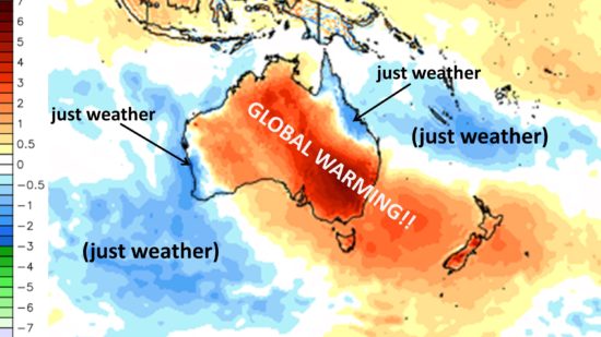
The Australian Bureau of Meteorology (BOM) claims January, 2019 was record-hot. There is no doubt it was very hot — but just how hot… and why?
The BOM announcement mentions “record” no less than 28 times… but nowhere (that I can find) in the report does it say just how long the historical record is. My understanding is that it is since 1910. So, of course, we have no idea what previous centuries might have shown for unusually hot summers.
The assumption is, of course, that anthropogenic global warming is to blame. But there is too much blaming of humans going on out there these days, when we know that natural weather fluctuations also cause record high (and low) temperatures, rainfall, etc.
But how is one to know what records are due to the human-component of global warming versus Mother Nature? (Even the UN IPCC admits some of the warming since the 1950s could be natural. Certainly, the warming from the Little Ice Age until 1940 was mostly natural.)
One characteristic of global warming is that it is (as the name implies) global — or nearly so (maybe not over Antarctica). In contrast, natural weather variations are regional, tied to natural variations and movements in atmospheric circulation systems.
That “weather” was strongly involved in the hot Australian January can be seen by the cooler than normal temperatures in coastal areas centered near Townsville in the northeast, and Perth in the southwest:
The extreme heat was caused by sinking air, which caused clear skies and record-low rainfall in some areas.
But why was the air sinking? It was being forced to sink by rising air in precipitation systems off-shore. All rising air must be exactly matched by an equal amount of sinking air, and places like Australia and the Sahara are naturally preferred for this — thus the arid and semi-arid environment. The heat originates from the latent heat release due to rain formation in those precipitation systems.
If we look at the area surrounding Australia in January, we can see just how localized the “record” warmth was. The snarky labels reflect my annoyance at people not thinking critically about the difference between ‘weather’ and ‘climate change’:
January 2019 surface temperature anomalies (deg. C, relative to the 1981-2010 average) from NOAA’s Global Forecast System (GFS) analysis fields. Unlabeled graphic courtesy of WeatherBell.com.
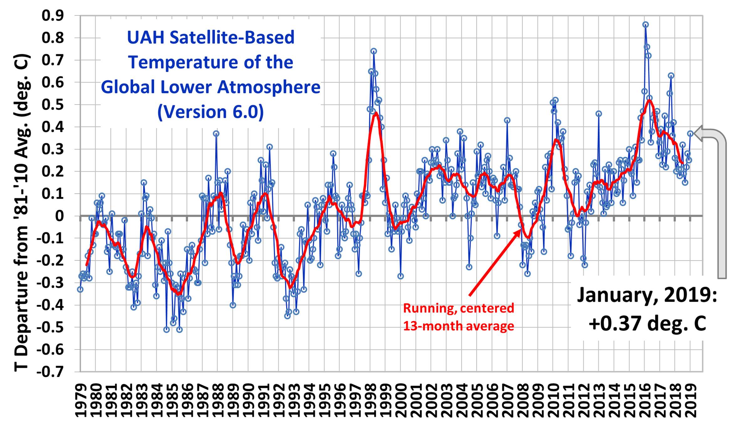
The Version 6.0 global average lower tropospheric temperature (LT) anomaly for January, 2019 was +0.37 deg. C, up from the December, 2018 value of +0.25 deg. C:
Global area-averaged lower tropospheric temperature anomalies (departures from 30-year calendar monthly means, 1981-2010). The 13-month centered average is meant to give an indication of the lower frequency variations in the data; the choice of 13 months is somewhat arbitrary… an odd number of months allows centered plotting on months with no time lag between the two plotted time series. The inclusion of two of the same calendar months on the ends of the 13 month averaging period causes no issues with interpretation because the seasonal temperature cycle has been removed, and so has the distinction between calendar months
Various regional LT departures from the 30-year (1981-2010) average for the last 13 months are:
The linear temperature trend of the global average lower tropospheric temperature anomalies from January 1979 through January 2019 remains at +0.13 C/decade.
The UAH LT global anomaly image for January, 2019 should be available in the next few days here.
The new Version 6 files should also be updated at that time, and are located here:
It’s much easier to devise and promote a climate change theory than it is to falsify it. Falsification requires a lot of data over a long period of time, something we don’t usually have in climate research.
The “polar vortex” is the deep cyclonic flow around a cold air mass generally covering the Arctic, Canada, and Northern Asia during winter. It is irregularly shaped, following the far-northern land masses, unlike it’s stratospheric cousin, which is often quite symmetric and centered on the North and South Poles.
For as long as we have had weather records (extending back into the 1800s), lobes of cold air rotating generally from west to east around the polar vortex sometimes extend down into the U.S. causing wild winter weather and general unpleasantness.
We used to call this process “weather”. Now it’s called “climate change”.
When these cold air outbreaks continued to menace the United States even as global warming has caused global average temperatures to creep upward, an explanation had to be found. After all, snow was supposed to be a thing of the past by now.
Enter the theory that decreasing wintertime sea ice cover in the Arctic (down about 15% over the last 40 years) has tended to displace the polar vortex in the general direction of southern Canuckistan and Yankeeland.
In other words, as the theory goes, global warming sometimes causes colder winters. This is what makes global warming theory so marvelously adaptable — it can explain anything.
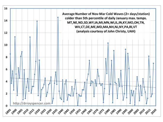
In the wake of the current cold wave, John Christy skated into my office this morning with a plot of U.S. winter cold waves since the late 1800s. He grouped the results by region, and examined cold waves lasting a minimum of 2 days at a station, and 5 days at a station. The results were basically the same.
As can be seen in the plot below, there is no evidence in the data supporting the claim that decreasing Arctic sea ice in recent decades is causing more frequent displacement of cold winter air masses into the eastern U.S., at least through the winter of 2017-18:
The trend is markedly downward in the most recent 40 years (since 1979) which is the earliest we have reliable measurements of Arctic sea ice from satellite microwave radiometers (my specialty).
Now, I suppose that Arctic sea ice decline could have some influence. But weather is immensely complex. Cause and effect is often difficult to ascertain.
At a minimum we should demand good observational support for any specific claim. In this case I would say that the connection between Eastern U.S. cold waves and Arctic sea ice is speculative, at best.
Yesterday I was reminded of this brilliant lecture by the late Dr. Michael Crichton, American author, screenwriter, director, and producer. Some of his more notable works include The Andromeda Strain (1969), Jurassic Park (1990), State of Fear (2004), The Great Train Robbery (1979), Twister (1996), and ER (1994-2009). John Christy and I were the basis for one of the characters in his book State of Fear.
Although I never met Dr. Crichton, he was immensely cordial and supportive of my first book when I had an email conversation with him, not long before his death in 2008. As I recall, he said he was dismayed that his 2005 congressional testimony led to so much criticism, and he was trying to avoid the subject going forward.
The themes in his 2003 lecture are just as relevant today as they were 16 years ago. I am told that some of of his works have been removed from the internet, possibly due to his controversial (non-PC) views on environmental matters. The lecture is lucid and concise, and echo the warning President Eisenhower gave in his 1961 Farewell Address about the government being in control of scientific research. I encourage you to spend 15 minutes reading it… there are gems throughout. (I have made made only very slight edits.)
Aliens Cause Global Warming
By Michael Crichton
Caltech Michelin Lecture January 17, 2003
My topic today sounds humorous but unfortunately I am serious. I am going to argue that extraterrestrials lie behind global warming. Or to speak more precisely, I will argue that a belief in extraterrestrials has paved the way, in a progression of steps, to a belief in global warming. Charting this progression of belief will be my task today.
Let me say at once that I have no desire to discourage anyone from believing in either extraterrestrials or global warming. That would be quite impossible to do. Rather, I want to discuss the history of several widely-publicized beliefs and to point to what I consider an emerging crisis in the whole enterprise of science — namely the increasingly uneasy relationship between hard science and public policy.
I have a special interest in this because of my own upbringing. I was born in the midst of World War II, and passed my formative years at the height of the Cold War. In school drills, I dutifully crawled under my desk in preparation for a nuclear attack.
It was a time of widespread fear and uncertainty, but even as a child I believed that science represented the best and greatest hope for mankind. Even to a child, the contrast was clear between the world of politics — a world of hate and danger, of irrational beliefs and fears, of mass manipulation and disgraceful blots on human history. In contrast, science held different values — international in scope, forging friendships and working relationships across national boundaries and political systems, encouraging a dispassionate habit of thought, and ultimately leading to fresh knowledge and technology that would benefit all mankind. The world might not be a very good place, but science would make it better. And it did. In my lifetime, science has largely fulfilled its promise. Science has been the great intellectual adventure of our age, and a great hope for our troubled and restless world. But I did not expect science merely to extend lifespan, feed the hungry, cure disease, and shrink the world with jets and cell phones. I also expected science to banish the evils of human thought — prejudice and superstition, irrational beliefs and false fears. I expected science to be, in Carl Sagan’s memorable phrase, “a candle in a demon haunted world.” And here, I am not so pleased with the impact of science. Rather than serving as a cleansing force, science has in some instances been seduced by the more ancient lures of politics and publicity. Some of the demons that haunt our world in recent years are invented by scientists. The world has not benefited from permitting these demons to escape free.
But let’s look at how it came to pass.
Cast your minds back to 1960. John F. Kennedy is president, commercial jet airplanes are just appearing, the biggest university mainframes have 12K of memory. And in Green Bank, West Virginia at the new National Radio Astronomy Observatory, a young astrophysicist named Frank Drake runs a two-week project called Ozma, to search for extraterrestrial signals. A signal is received, to great excitement. It turns out to be false, but the excitement remains. In 1960, Drake organizes the first SETI conference, and came up with the now-famous Drake equation:
N=R*fp*ne*fl*fi*fc*fL
[where R is the number of stars in the Milky Way galaxy; fp is the fraction with planets; ne is the number of planets per star capable of supporting life; fl is the fraction of planets where life evolves; fi is the fraction where intelligent life evolves; and fc is the fraction that communicates; and fL is the fraction of the planet’s life during which the communicating civilizations live.]
This serious-looking equation gave SETI a serious footing as a legitimate intellectual inquiry. The problem, of course, is that none of the terms can be known, and most cannot even be estimated. The only way to work the equation is to fill in with guesses. And guesses — just so we’re clear — are merely expressions of prejudice. Nor can there be “informed guesses.” If you need to state how many planets with life choose to communicate, there is simply no way to make an informed guess. It’s simply prejudice.
As a result, the Drake equation can have any value from “billions and billions” to zero. An expression that can mean anything means nothing. Speaking precisely, the Drake equation is literally meaningless, and has nothing to do with science. I take the hard view that science involves the creation of testable hypotheses. The Drake equation cannot be tested and therefore SETI is not science. SETI is unquestionably a religion. Faith is defined as the firm belief in something for which there is no proof. The belief that the Koran is the word of God is a matter of faith. The belief that God created the universe in seven days is a matter of faith. The belief that there are other life forms in the universe is a matter of faith. There is not a single shred of evidence for any other life forms, and in forty years of searching, none has been discovered. There is absolutely no evidentiary reason to maintain this belief. SETI is a religion.
One way to chart the cooling of enthusiasm is to review popular works on the subject. In 1964, at the height of SETI enthusiasm, Walter Sullivan of the NY Times wrote an exciting book about life in the universe entitled WE ARE NOT ALONE. By 1995, when Paul Davis wrote a book on the same subject, he titled it ARE WE ALONE? ( Since 1981, there have in fact been four books titled ARE WE ALONE.) More recently we have seen the rise of the so-called “Rare Earth” theory which suggests that we may, in fact, be all alone. Again, there is no evidence either way.
Back in the sixties, SETI had its critics, although not among astrophysicists and astronomers. The biologists and paleontologists were harshest. George Gaylord Simpson of Harvard sneered that SETI was a “study without a subject,” and it remains so to the present day. But scientists in general have been indulgent toward SETI, viewing it either with bemused tolerance, or with indifference. After all, what’s the big deal? It’s kind of fun. If people want to look, let them. Only a curmudgeon would speak harshly of SETI. It wasn’t worth the bother.
And of course, it is true that untestable theories may have heuristic value. Of course, extraterrestrials are a good way to teach science to kids. But that does not relieve us of the obligation to see the Drake equation clearly for what it is — pure speculation in quasi-scientific trappings.
The fact that the Drake equation was not greeted with screams of outrage —similar to the screams of outrage that greet each Creationist new claim, for example — meant that now there was a crack in the door, a loosening of the definition of what constituted legitimate scientific procedure. And soon enough, pernicious garbage began to squeeze through the cracks.
Now let’s jump ahead a decade to the 1970s, and Nuclear Winter.
In 1975, the National Academy of Sciences reported on “Long-Term Worldwide Effects of Multiple Nuclear Weapons Detonations” but the report estimated the effect of dust from nuclear blasts to be relatively minor. In 1979, the Office of Technology Assessment issued a report on “The Effects of Nuclear War” and stated that nuclear war could perhaps produce irreversible adverse consequences on the environment. However, because the scientific processes involved were poorly understood, the report stated it was not possible to estimate the probable magnitude of such damage.
Three years later, in 1982, the Swedish Academy of Sciences commissioned a report entitled “The Atmosphere after a Nuclear War: Twilight at Noon,” which attempted to quantify the effect of smoke from burning forests and cities. The authors speculated that there would be so much smoke that a large cloud over the northern hemisphere would reduce incoming sunlight below the level required for photosynthesis, and that this would last for weeks or even longer.
The following year, five scientists including Richard Turco and Carl Sagan published a paper in Science called “Nuclear Winter: Global Consequences of Multiple Nuclear Explosions.” This was the so-called TTAPS report, which attempted to quantify more rigorously the atmospheric effects, with the added credibility to be gained from an actual computer model of climate.
At the heart of the TTAPS undertaking was another equation, never specifically expressed, but one that could be paraphrased as follows:
Ds = Wn*Ws*Wh*T*Tb*Pt*Pr*Pe, etc.
(The amount of tropospheric dust = # warheads x size warheads x warhead detonation height x flammability of targets x Target burn duration x Particles entering the Troposphere x Particle reflectivity x Particle endurance, and so on.)
The similarity to the Drake equation is striking. As with the Drake equation, none of the variables can be determined. None at all. The TTAPS study addressed this problem in part by mapping out different wartime scenarios and assigning numbers to some of the variables, but even so, the remaining variables were — and are — simply unknowable. Nobody knows how much smoke will be generated when cities burn, creating particles of what kind, and for how long. No one knows the effect of local weather conditions on the amount of particles that will be injected into the troposphere. No one knows how long the particles will remain in the troposphere. And so on.
And remember, this is only four years after the OTA study concluded that the underlying scientific processes were so poorly known that no estimates could be reliably made. Nevertheless, the TTAPS study not only made those estimates, but concluded they were catastrophic.
According to Sagan and his coworkers, even a limited 5,000 megaton nuclear exchange would cause a global temperature drop of more than 35 degrees Centigrade, and this change would last for three months. The greatest volcanic eruptions that we know of changed world temperatures somewhere between 0.5 and 2 degrees Centigrade. Ice ages changed global temperatures by 10 degrees. Here we have an estimated change three times greater than any ice age. One might expect it to be the subject of some dispute.
But Sagan and his coworkers were prepared, for nuclear winter was from the outset the subject of a well-orchestrated media campaign. The first announcement of nuclear winter appeared in an article by Sagan in the Sunday supplement, Parade. The very next day, a highly-publicized, high-profile conference on the long-term consequences of nuclear war was held in Washington, chaired by Carl Sagan and Paul Ehrlich, the most famous and media-savvy scientists of their generation. Sagan appeared on the Johnny Carson show 40 times. Ehrlich was on 25 times. Following the conference, there were press conferences, meetings with congressmen, and so on. The formal papers in Science came months later.
This is not the way science is done, it is the way products are sold.
The real nature of the conference is indicated by these artists’ renderings of the effect of nuclear winter.
I cannot help but quote the caption for figure 5: “Shown here is a tranquil scene in the north woods. A beaver has just completed its dam, two black bears forage for food, a swallow-tailed butterfly flutters in the foreground, a loon swims quietly by, and a kingfisher searches for a tasty fish.” Hard science if ever there was.
At the conference in Washington, during the question period, Ehrlich was reminded that after Hiroshima and Nagasaki, scientists were quoted as saying nothing would grow there for 75 years, but in fact melons were growing the next year. So, he was asked, how accurate were these findings now?
Ehrlich answered by saying “I think they are extremely robust. Scientists may have made statements like that, although I cannot imagine what their basis would have been, even with the state of science at that time, but scientists are always making absurd statements, individually, in various places. What we are doing here, however, is presenting a consensus of a very large group of scientists.”
I want to pause here and talk about this notion of consensus, and the rise of what has been called consensus science. I regard consensus science as an extremely pernicious development that ought to be stopped cold in its tracks. Historically, the claim of consensus has been the first refuge of scoundrels; it is a way to avoid debate by claiming that the matter is already settled.
Whenever you hear the consensus of scientists agrees on something or other, reach for your wallet, because you’re being had.
Let’s be clear: the work of science has nothing whatever to do with consensus. Consensus is the business of politics. Science, on the contrary, requires only one investigator who happens to be right, which means that he or she has results that are verifiable by reference to the real world. In science consensus is irrelevant. What is relevant is reproducible results. The greatest scientists in history are great precisely because they broke with the consensus.
There is no such thing as consensus science. If it’s consensus, it isn’t science. If it’s science, it isn’t consensus. Period.
In addition, let me remind you that the track record of the consensus is nothing to be proud of. Let’s review a few cases.
In past centuries, the greatest killer of women was fever following childbirth . One woman in six died of this fever. In 1795, Alexander Gordon of Aberdeen suggested that the fevers were infectious processes, and he was able to cure them. The consensus said no. In 1843, Oliver Wendell Holmes claimed puerperal fever was contagious, and presented compelling evidence. The consensus said no. In 1849, Semmelweiss demonstrated that sanitary techniques virtually eliminated puerperal fever in hospitals under his management. The consensus said he was a Jew, ignored him, and dismissed him from his post. There was in fact no agreement on puerperal fever until the start of the twentieth century. Thus the consensus took one hundred and twenty five years to arrive at the right conclusion despite the efforts of the prominent “skeptics” around the world, skeptics who were demeaned and ignored. And despite the constant ongoing deaths of women.
There is no shortage of other examples. In the 1920s in America, tens of thousands of people, mostly poor, were dying of a disease called pellagra. The consensus of scientists said it was infectious, and what was necessary was to find the “pellagra germ.” The US government asked a brilliant young investigator, Dr. Joseph Goldberger, to find the cause. Goldberger concluded that diet was the crucial factor. The consensus remained wedded to the germ theory. Goldberger demonstrated that he could induce the disease through diet. He demonstrated that the disease was not infectious by injecting the blood of a pellagra patient into himself, and his assistant. They and other volunteers swabbed their noses with swabs from pellagra patients, and swallowed capsules containing scabs from pellagra rashes in what were called “Goldberger’s filth parties.” Nobody contracted pellagra. The consensus continued to disagree with him. There was, in addition, a social factor — southern States disliked the idea of poor diet as the cause, because it meant that social reform was required. They continued to deny it until the 1920s. Result — despite a twentieth century epidemic, the consensus took years to see the light.
Probably every schoolchild notices that South America and Africa seem to fit together rather snugly, and Alfred Wegener proposed, in 1912, that the continents had in fact drifted apart. The consensus sneered at continental drift for fifty years. The theory was most vigorously denied by the great names of geology — until 1961, when it began to seem as if the sea floors were spreading. The result: it took the consensus fifty years to acknowledge what any schoolchild sees.
And shall we go on? The examples can be multiplied endlessly. Jenner and smallpox, Pasteur and germ theory. Saccharine, margarine, repressed memory, fiber and colon cancer, hormone replacement therapy. The list of consensus errors goes on and on.
Finally, I would remind you to notice where the claim of consensus is invoked. Consensus is invoked only in situations where the science is not solid enough. Nobody says the consensus of scientists agrees that E=mc2 . Nobody says the consensus is that the sun is 93 million miles away. It would never occur to anyone to speak that way.
But back to our main subject.
What I have been suggesting to you is that nuclear winter was a meaningless formula, tricked out with bad science, for policy ends. It was political from the beginning, promoted in a well-orchestrated media campaign that had to be planned weeks or months in advance.
Further evidence of the political nature of the whole project can be found in the response to criticism. Although Richard Feynman was characteristically blunt, saying, “I really don’t think these guys know what they’re talking about,” other prominent scientists were noticeably reticent. Freeman Dyson was quoted as saying “It’s an absolutely atrocious piece of science but who wants to be accused of being in favor of nuclear war?” And Victor Weisskopf said, “The science is terrible but — perhaps the psychology is good.” The nuclear winter team followed up the publication of such comments with letters to the editors denying that these statements were ever made, though the scientists since then have subsequently confirmed their views.
At the time, there was a concerted desire on the part of lots of people to avoid nuclear war. If nuclear winter looked awful, why investigate too closely? Who wanted to disagree? Only people like Edward Teller, the “father of the H bomb.”
Teller said, “While it is generally recognized that details are still uncertain and deserve much more study, Dr. Sagan nevertheless has taken the position that the whole scenario is so robust that there can be little doubt about its main conclusions.” Yet for most people, the fact that nuclear winter was a scenario riddled with uncertainties did not seem to be relevant.
I say it is hugely relevant. Once you abandon strict adherence to what science tells us, once you start arranging the truth in a press conference, then anything is possible. In one context, maybe you will get some mobilization against nuclear war. But in another context, you get Lysenkoism. In another, you get Nazi euthanasia. The danger is always there, if you subvert science to political ends.
That is why it is so important for the future of science that the line between what science can say with certainty, and what it cannot, be drawn clearly — and defended.
What happened to Nuclear Winter? As the media glare faded, its robust scenario appeared less persuasive; John Maddox, editor of Nature, repeatedly criticized its claims; within a year, Stephen Schneider, one of the leading figures in the climate model, began to speak of “nuclear autumn.” It just didn’t have the same ring.
A final media embarrassment came in 1991, when Carl Sagan predicted on Nightline that Kuwaiti oil fires would produce a nuclear winter effect, causing a “year without a summer,” and endangering crops around the world. Sagan stressed this outcome was so likely that “it should affect the war plans.” None of it happened.
What, then, can we say were the lessons of Nuclear Winter? I believe the lesson was that with a catchy name, a strong policy position and an aggressive media campaign, nobody will dare to criticize the science, and in short order, a terminally weak thesis will be established as fact. After that, any criticism becomes beside the point. The war is already over without a shot being fired. That was the lesson, and we had a textbook application soon afterward, with second hand smoke.
In 1993, the EPA announced that second-hand smoke was “responsible for approximately 3,000 lung cancer deaths each year in nonsmoking adults,” and that it “impairs the respiratory health of hundreds of thousands of people.” In a 1994 pamphlet the EPA said that the eleven studies it based its decision on were not by themselves conclusive, and that they collectively assigned second-hand smoke a risk factor of 1.19. (For reference, a risk factor below 3.0 is too small for action by the EPA. or for publication in the New England Journal of Medicine, for example.) Furthermore, since there was no statistical association at the 95% confidence limits, the EPA lowered the limit to 90%. They then classified second-hand smoke as a Group-A Carcinogen.
This was openly fraudulent science, but it formed the basis for bans on smoking in restaurants, offices, and airports. California banned public smoking in 1995. Soon, no claim was too extreme. By 1998, the Christian Science Monitor was saying that “Second-hand smoke is the nation’s third-leading preventable cause of death.” The American Cancer Society announced that 53,000 people died each year of second-hand smoke. The evidence for this claim is nonexistent.
In 1998, a Federal judge held that the EPA had acted improperly, had “committed to a conclusion before research had begun,” and had “disregarded information and made findings on selective information.” The reaction of Carol Browner, head of the EPA was: “We stand by our science; there’s wide agreement. The American people certainly recognize that exposure to second hand smoke brings a whole host of health problems.” Again, note how the claim of consensus trumps science. In this case, it isn’t even a consensus of scientists that Browner evokes! It’s the consensus of the American people.
Meanwhile, ever-larger studies failed to confirm any association. A large, seven-country WHO study in 1998 found no association. Nor have well-controlled subsequent studies, to my knowledge. Yet we now read, for example, that second-hand smoke is a cause of breast cancer. At this point you can say pretty much anything you want about second-hand smoke.
As with nuclear winter, bad science is used to promote what most people would consider good policy. I certainly think it is. I don’t want people smoking around me. So who will speak out against banning second-hand smoke? Nobody, and if you do, you’ll be branded a shill of RJ Reynolds. A big tobacco flunky. But the truth is that we now have a social policy supported by the grossest of superstitions. And we’ve given the EPA a bad lesson in how to behave in the future. We’ve told them that cheating is the way to succeed.
As the twentieth century drew to a close, the connection between hard scientific fact and public policy became increasingly elastic. In part this was possible because of the complacency of the scientific profession; in part because of the lack of good science education among the public; in part, because of the rise of specialized advocacy groups which have been enormously effective in getting publicity and shaping policy; and in great part because of the decline of the media as an independent assessor of fact. The deterioration of the American media is dire loss for our country. When distinguished institutions like the New York Times can no longer differentiate between factual content and editorial opinion, but rather mix both freely on their front page, then who will hold anyone to a higher standard?
And so, in this elastic anything-goes world where science — or non-science — is the hand maiden of questionable public policy, we arrive at last at global warming. It is not my purpose here to rehash the details of this most magnificent of the demons haunting the world. I would just remind you of the now-familiar pattern by which these things are established. Evidentiary uncertainties are glossed over in the unseemly rush for an overarching policy, and for grants to support the policy by delivering findings that are desired by the patron. Next, the isolation of those scientists who won’t get with the program, and the characterization of those scientists as outsiders and “skeptics” in quotation marks — suspect individuals with suspect motives, industry flunkies, reactionaries, or simply anti-environmental nut-cases. In short order, debate ends, even though prominent scientists are uncomfortable about how things are being done.
When did “skeptic” become a dirty word in science? When did a skeptic require quotation marks around it?
To an outsider, the most significant innovation in the global warming controversy is the overt reliance that is being placed on models. Back in the days of nuclear winter, computer models were invoked to add weight to a conclusion: “These results are derived with the help of a computer model.” But now, large-scale computer models are seen as generating data in themselves. No longer are models judged by how well they reproduce data from the real world — increasingly, models provide the data. As if they were themselves a reality. And indeed they are, when we are projecting forward. There can be no observational data about the year 2100. There are only model runs.
This fascination with computer models is something I understand very well. Richard Feynmann called it a disease. I fear he is right. Because only if you spend a lot of time looking at a computer screen can you arrive at the complex point where the global warming debate now stands.
Nobody believes a weather prediction twelve hours ahead. Now we’re asked to believe a prediction that goes out 100 years into the future? And make financial investments based on that prediction? Has everybody lost their minds?
Stepping back, I have to say the arrogance of the model-makers is breathtaking. There have been, in every century, scientists who say they know it all. Since climate may be a chaotic system — no one is sure — these predictions are inherently doubtful, to be polite. But more to the point, even if the models get the science spot-on, they can never get the sociology. To predict anything about the world a hundred years from now is simply absurd.
Look: If I was selling stock in a company that I told you would be profitable in 2100, would you buy it? Or would you think the idea was so crazy that it must be a scam?
Let’s think back to people in 1900 in, say, New York. If they worried about people in 2000, what would they worry about? Probably: Where would people get enough horses? And what would they do about all the horseshit? Horse pollution was bad in 1900, think how much worse it would be a century later, with so many more people riding horses?
But of course, within a few years, nobody rode horses except for sport. And in 2000, France was getting 80% its power from an energy source that was unknown in 1900. Germany, Switzerland, Belgium and Japan were getting more than 30% from this source, unknown in 1900. Remember, people in 1900 didn’t know what an atom was. They didn’t know its structure. They also didn’t know what a radio was, or an airport, or a movie, or a television, or a computer, or a cell phone, or a jet, an antibiotic, a rocket, a satellite, an MRI, ICU, IUD, IBM, IRA, ERA, EEG, EPA, IRS, DOD, PCP, HTML, internet, interferon, instant replay, remote sensing, remote control, speed dialing, gene therapy, gene splicing, genes, spot welding, heat-seeking, bipolar, prozac, leotards, lap dancing, email, tape recorder, CDs, airbags, plastic explosive, plastic, robots, cars, liposuction, transduction, superconduction, dish antennas, step aerobics, smoothies, twelve-step, ultrasound, nylon, rayon, teflon, fiber optics, carpal tunnel, laser surgery, laparoscopy, corneal transplant, kidney transplant, AIDS. None of this would have meant anything to a person in the year 1900. They wouldn’t know what you are talking about.
Now. You tell me you can predict the world of 2100. Tell me it’s even worth thinking about. Our models just carry the present into the future. They’re bound to be wrong. Everybody who gives a moment’s thought knows it.
I remind you that in the lifetime of most scientists now living, we have already had an example of dire predictions set aside by new technology. I refer to the green revolution. In 1960, Paul Ehrlich said, “The battle to feed humanity is over. In the 1970s the world will undergo famines — hundreds of millions of people are going to starve to death.” Ten years later, he predicted four billion people would die during the 1980s, including 65 million Americans. The mass starvation that was predicted never occurred, and it now seems it isn’t ever going to happen. Nor is the population explosion going to reach the numbers predicted even ten years ago. In 1990, climate modelers anticipated a world population of 11 billion by 2100. Today, some people think the correct number will be 7 billion and falling. But nobody knows for sure.
But it is impossible to ignore how closely the history of global warming fits on the previous template for nuclear winter. Just as the earliest studies of nuclear winter stated that the uncertainties were so great that probabilities could never be known, so, too the first pronouncements on global warming argued strong limits on what could be determined with certainty about climate change. The 1995 IPCC draft report said, “Any claims of positive detection of significant climate change are likely to remain controversial until uncertainties in the total natural variability of the climate system are reduced.” It also said, “No study to date has positively attributed all or part of observed climate changes to anthropogenic causes.” Those statements were removed, and in their place appeared: “The balance of evidence suggests a discernable human influence on climate.”
What is clear, however, is that on this issue, science and policy have become inextricably mixed to the point where it will be difficult, if not impossible, to separate them out. It is possible for an outside observer to ask serious questions about the conduct of investigations into global warming, such as whether we are taking appropriate steps to improve the quality of our observational data records, whether we are systematically obtaining the information that will clarify existing uncertainties, whether we have any organized disinterested mechanism to direct research in this contentious area.
The answer to all these questions is no. We don’t.
In trying to think about how these questions can be resolved, it occurs to me that in the progression from SETI to nuclear winter to second-hand smoke to global warming, we have one clear message, and that is that we can expect more and more problems of public policy dealing with technical issues in the future — problems of ever greater seriousness, where people care passionately on all sides.
And at the moment we have no mechanism to get good answers. So I will propose one.
Just as we have established a tradition of double-blinded research to determine drug efficacy, we must institute double-blinded research in other policy areas as well. Certainly the increased use of computer models, such as GCMs, cries out for the separation of those who make the models from those who verify them. The fact is that the present structure of science is entrepreneurial, with individual investigative teams vying for funding from organizations that all too often have a clear stake in the outcome of the research — or appear to, which may be just as bad. This is not healthy for science.
Sooner or later, we must form an independent research institute in this country. It must be funded by industry, by government, and by private philanthropy, both individuals and trusts. The money must be pooled, so that investigators do not know who is paying them. The institute must fund more than one team to do research in a particular area, and the verification of results will be a foregone requirement: teams will know their results will be checked by other groups. In many cases, those who decide how to gather the data will not gather it, and those who gather the data will not analyze it. If we were to address the land temperature records with such rigor, we would be well on our way to an understanding of exactly how much faith we can place in global warming, and therefore with what seriousness we must address this.
I believe that as we come to the end of this litany, some of you may be saying, well what is the big deal, really. So we made a few mistakes. So a few scientists have overstated their cases and have egg on their faces. So what?
Well, I’ll tell you.
In recent years, much has been said about the post-modernist claims about science to the effect that science is just another form of raw power, tricked out in special claims for truth-seeking and objectivity that really have no basis in fact. Science, we are told, is no better than any other undertaking. These ideas anger many scientists, and they anger me. But recent events have made me wonder if they are correct. We can take as an example the scientific reception accorded a Danish statistician, Bjorn Lomborg, who wrote a book called The Skeptical Environmentalist.
The scientific community responded in a way that can only be described as disgraceful. In professional literature, it was complained he had no standing because he was not an earth scientist. His publisher, Cambridge University Press, was attacked with cries that the editor should be fired, and that all right-thinking scientists should shun the press. The past president of the AAAS wondered aloud how Cambridge could have ever “published a book that so clearly could never have passed peer review.” (But of course, the manuscript did pass peer review by three earth scientists on both sides of the Atlantic, and all recommended publication.) But what are scientists doing attacking a press? Is this the new McCarthyism — coming from scientists?
Worst of all was the behavior of the Scientific American, which seemed intent on proving the post-modernist point that it was all about power, not facts. The Scientific American attacked Lomborg for eleven pages, yet only came up with nine factual errors despite their assertion that the book was “rife with careless mistakes.” It was a poor display, featuring vicious ad hominem attacks, including comparing him to a Holocaust denier. The issue was captioned: “Science defends itself against the Skeptical Environmentalist.” Really. Science has to defend itself? Is this what we have come to?
When Lomborg asked for space to rebut his critics, he was given only a page and a half. When he said it wasn’t enough, he put the critics’ essays on his web page and answered them in detail. Scientific American threatened copyright infringement and made him take the pages down.
Further attacks since, have made it clear what is going on. Lomborg is charged with heresy. That’s why none of his critics needs to substantiate their attacks in any detail. That’s why the facts don’t matter. That’s why they can attack him in the most vicious personal terms. He’s a heretic.
Of course, any scientist can be charged as Galileo was charged. I just never thought I’d see the Scientific American in the role of Mother Church.
Is this what science has become? I hope not. But it is what it will become, unless there is a concerted effort by leading scientists to aggressively separate science from policy. The late Philip Handler, former president of the National Academy of Sciences, said that “Scientists best serve public policy by living within the ethics of science, not those of politics. If the scientific community will not unfrock the charlatans, the public will not discern the difference — science and the nation will suffer.”
Personally, I don’t worry about the nation. But I do worry about science.
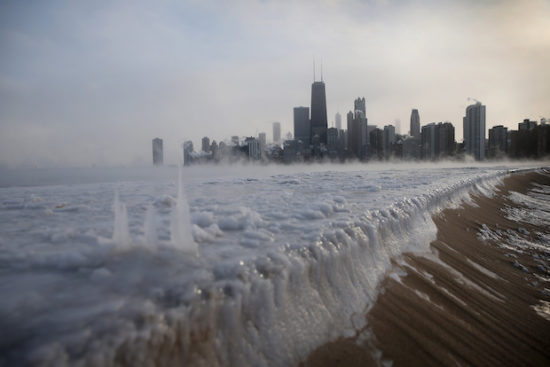
Lake Michigan ice as temperatures plunged to -16 deg. F in Chicago, IL on Jan. 6, 2014. The low temperature on Wednesday, January 30, 2019 could approach -30 deg F in the Chicago suburbs. (Getty Images)
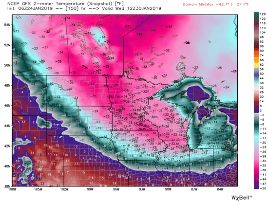
A “Siberian Express” weather disturbance currently crossing the Arctic Ocean will meet up with the semi-permanent winter “polar vortex” over Canada, pushing a record-breaking cold air mass into the Upper Plains and Midwest U.S. by Wednesday.
Chicago All-Time Record Low?
Both the European (ECMWF) and U.S. (GFS) weather forecast models are in agreement that by Wednesday morning temperatures in the Chicago suburbs will be approaching -30 deg. F. The all-time official record low for the Chicago metro area was -27 deg. F (O’Hare) on January 20, 1985, and that 34 year old record could fall as the ECMWF model is forecasting -32 deg. F for Thursday morning while the GFS model is bottoming out at -26 deg. F on Wednesday morning. Of course, these forecasts will change somewhat in the coming days as the cold wave approaches.
Dangerous Wind Chills
Like the record-breaking event of January 1985, the frigid temperatures will be accompanied by strong winds — gusting to 20 to 30 mph — with wind chills plunging to -60 deg. F at times. This is dangerously cold, and I suspect schools will close, water lines will freeze, and travel will be discouraged. Again, this event is still several days away, but the public should be aware of the potential severity of this cold wave.
Not Just Chicago
The GFS forecast temperatures for Wednesday morning shows most of the upper Midwest will be well below zero, and temperatures might not get above -20 deg. F even at midday on Wednesday as far south as northern Indiana. Again, the strong northwest winds will be pushing this air southeast, and Thursday morning will also bring record-breaking cold into the Ohio River Valley.
Forecast temperatures Wednesday morning, January 30, 2019 from the GFS model. (Graphic courtesy of WeatherBell.com).
I’ve been wanting to do this kind of time lapse of a lunar eclipse to show just how much change in brightness occurs when the full moon suddenly becomes nearly dark.
Most presentations of a lunar eclipse don’t really capture the darkening, just the change in color as the moon transitions from being illuminated by direct sunlight to the weak sunset glow from the annulus of scattered sunlight through Earth’s atmosphere.
I took three hours of photos, one every 23 seconds, at Little River Canyon, Alabama to make this. The camera setting was constant throughout (ISO640, f/5.6, 20 sec exposures). The temperature was unusually cold, 26 deg. F, low humidity, and there was a moderate wind out of the north. The video is best appreciated full-screen.
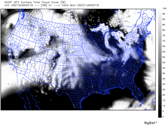
Tomorrow night (January 20-21) will present the whole U.S. with a total lunar eclipse, the best one until May 15, 2022.
Totality here in Alabama will occur approximately from 10:40 to 11:40 p.m. CST. Clear weather will be restricted mostly to the southeastern U.S., and portions of the Northern Plains and Great Lakes:
A Mystery (to me, anyway)
There’s one aspect of the eclipse I cannot figure out. I’m sure the explanation will be simple, and when someone explains it to me, my response will be, “DOH!”.
The illumination of the moon during totality is due to light scattered through Earth’s atmosphere. Just as we see red sunsets, that red light will be shining on the moon from an annulus of red sunset light circling the Earth.
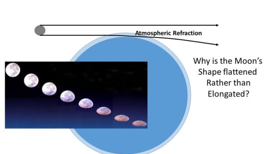
What I don’t understand, though, is the role of sunlight refraction (bending of sunlight) as it passes through the atmosphere at an oblique angle. The refraction occurs whether it is the moon or the sun being viewed through the limb, and I will use the example of moonlight shining through the limb.
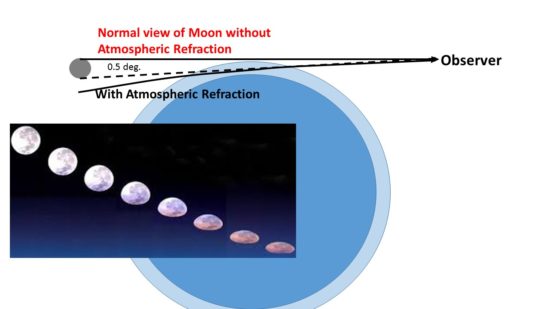
My understanding is that light (from either the moon or sun) bends as I crudely show in the following cartoon. The “mystery” arises from the fact that we know that the appearance of the moon is that it is flattened due to refraction (this is NOT a diagram of what is happening during the eclipse.. it’s a general question about how either sunlight or moonlight is refracted as it passes close to Earth’s limb):
The moon composite photo is from the ISS, so it is exactly analogous to the situation shown in the drawing.
So, the mystery: Why is the moon flattened rather elongated? I simply don’t know. But I’m sure the explanation is simple.
Update: Mystery Solved
As I suspected, the problem was in the way I was looking at it. As Brent Auvermann suggests in the comments, here’s the proper way to look at it. The eye sees the top and bottom of the moon at 2 slightly different angles, which are normally separated by 0.5 deg. But when the view in the direction of the bottom of the moon (0.5 deg. below the top of the moon) goes through a lot of atmosphere, it gets refracted downward, and the view from that direction comes from below the moon. In other words, what is a 0.5 degree subtended angle viewed by the eye actually originates from a bigger angle than that on the other side of the Earth’s limb. That causes the bottom of the moon to be compressed into a smaller angle (flattened):

 Home/Blog