Home/Blog
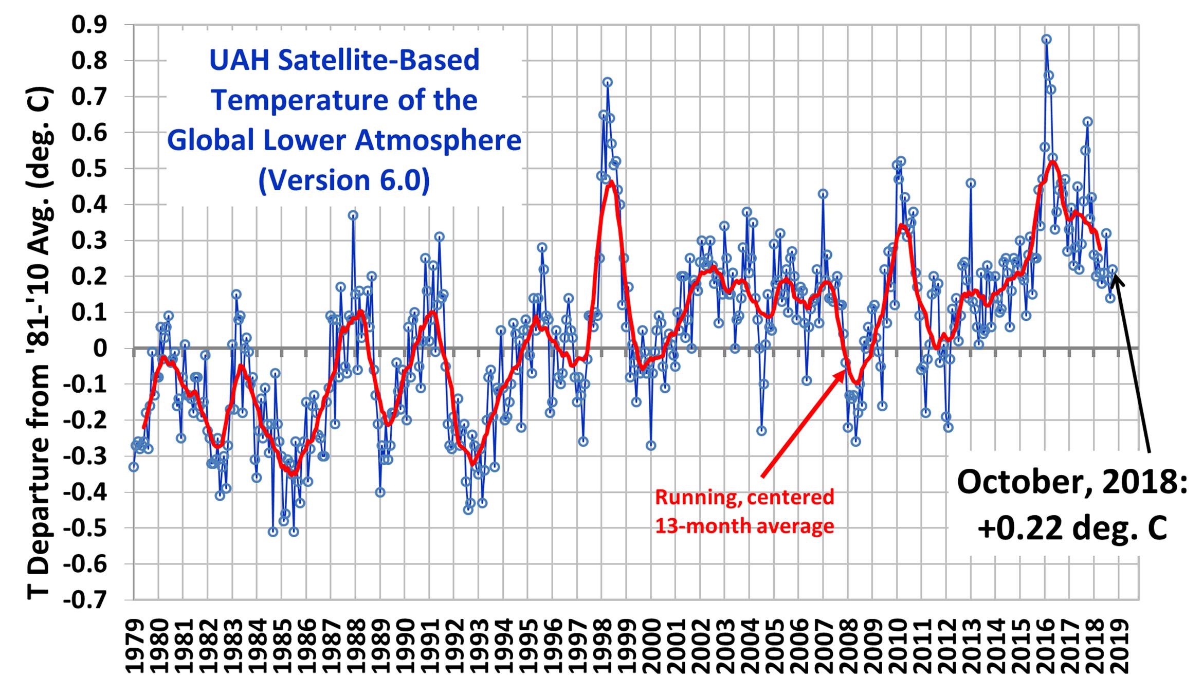
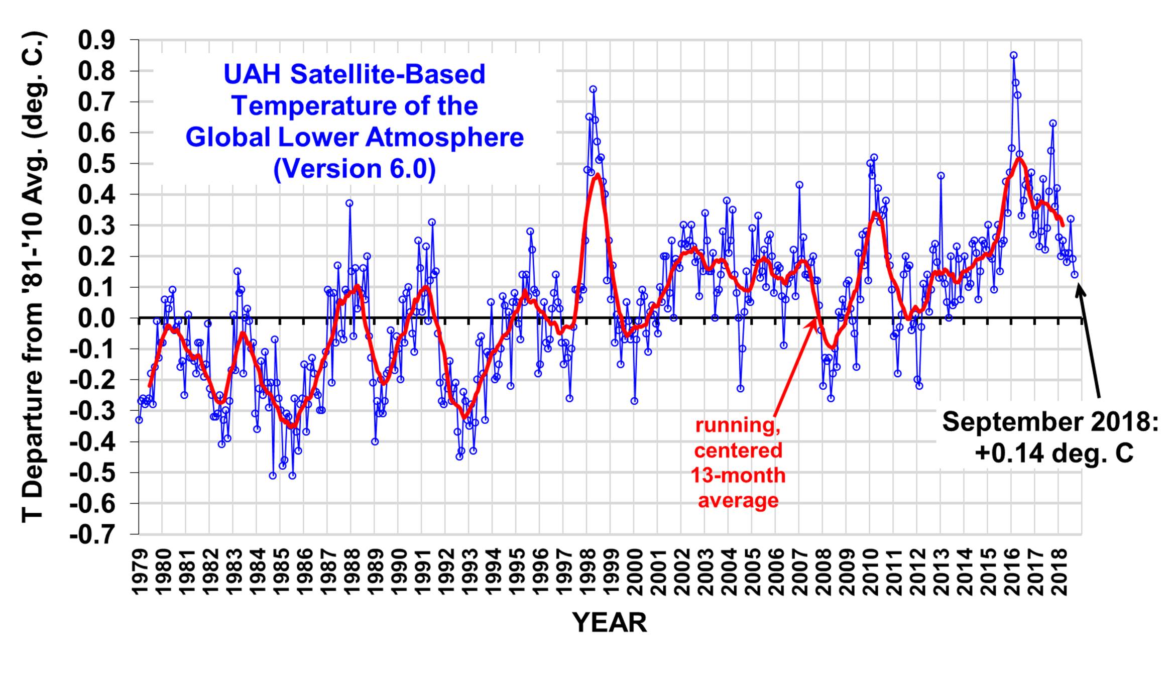
The Version 6.0 global average lower tropospheric temperature (LT) anomaly for November, 2018 was +0.28 deg. C, up a little from +0.22 deg. C in October:
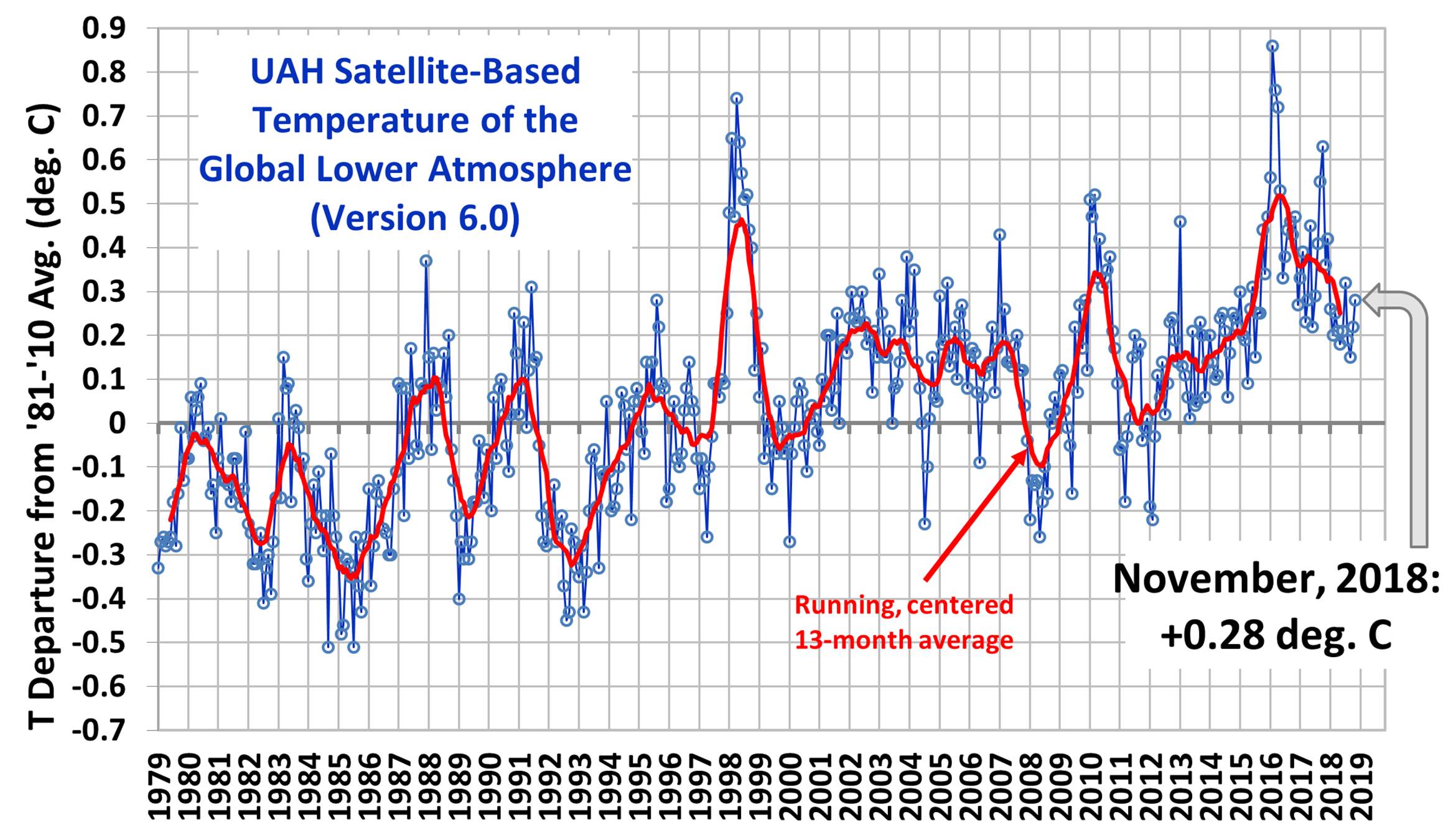
Global area-averaged lower tropospheric temperature anomalies (departures from 30-year calendar monthly means, 1981-2010). The 13-month centered average is meant to give an indication of the lower frequency variations in the data; the choice of 13 months is somewhat arbitrary… an odd number of months allows centered plotting on months with no time lag between the two plotted time series. The inclusion of two of the same calendar months on the ends of the 13 month averaging period causes no issues with interpretation because the seasonal temperature cycle has been removed, and so has the distinction between calendar months.
Various regional LT departures from the 30-year (1981-2010) average for the last 23 months are:
YEAR MO GLOBE NHEM. SHEM. TROPIC USA48 ARCTIC AUST
2017 01 +0.33 +0.32 +0.34 +0.10 +0.28 +0.95 +1.22
2017 02 +0.39 +0.58 +0.20 +0.08 +2.16 +1.33 +0.21
2017 03 +0.23 +0.37 +0.09 +0.06 +1.22 +1.24 +0.98
2017 04 +0.28 +0.29 +0.27 +0.22 +0.90 +0.23 +0.40
2017 05 +0.45 +0.40 +0.50 +0.41 +0.11 +0.21 +0.06
2017 06 +0.22 +0.34 +0.10 +0.40 +0.51 +0.10 +0.34
2017 07 +0.29 +0.31 +0.28 +0.51 +0.61 -0.27 +1.03
2017 08 +0.41 +0.41 +0.42 +0.47 -0.54 +0.49 +0.78
2017 09 +0.55 +0.52 +0.58 +0.54 +0.30 +1.06 +0.60
2017 10 +0.63 +0.67 +0.60 +0.48 +1.22 +0.83 +0.86
2017 11 +0.36 +0.34 +0.38 +0.27 +1.36 +0.68 -0.12
2017 12 +0.42 +0.50 +0.33 +0.26 +0.45 +1.37 +0.36
2018 01 +0.26 +0.46 +0.06 -0.11 +0.59 +1.36 +0.43
2018 02 +0.20 +0.25 +0.16 +0.03 +0.92 +1.20 +0.18
2018 03 +0.25 +0.40 +0.10 +0.07 -0.31 -0.32 +0.60
2018 04 +0.21 +0.32 +0.11 -0.12 -0.00 +1.02 +0.69
2018 05 +0.18 +0.41 -0.05 +0.03 +1.94 +0.18 -0.39
2018 06 +0.21 +0.38 +0.04 +0.12 +1.20 +0.83 -0.55
2018 07 +0.32 +0.43 +0.21 +0.29 +0.51 +0.30 +1.37
2018 08 +0.19 +0.22 +0.17 +0.12 +0.07 +0.09 +0.26
2018 09 +0.15 +0.15 +0.14 +0.24 +0.88 +0.21 +0.19
2018 10 +0.22 +0.31 +0.12 +0.34 +0.25 +1.11 +0.39
2018 11 +0.28 +0.27 +0.29 +0.50 -1.13 +0.69 +0.53
The linear temperature trend of the global average lower tropospheric temperature anomalies from January 1979 through November 2018 remains at +0.13 C/decade.
The UAH LT global anomaly image for November, 2018 should be available in the next few days here.
The new Version 6 files should also be updated at that time, and are located here:
Lower Troposphere: http://vortex.nsstc.uah.edu/data/msu/v6.0/tlt/uahncdc_lt_6.0.txt
Mid-Troposphere: http://vortex.nsstc.uah.edu/data/msu/v6.0/tmt/uahncdc_mt_6.0.txt
Tropopause: http://vortex.nsstc.uah.edu/data/msu/v6.0/ttp/uahncdc_tp_6.0.txt
Lower Stratosphere: http://vortex.nsstc.uah.edu/data/msu/v6.0/tls/uahncdc_ls_6.0.txt