Today marks the 25th anniversary of the tornado that tore through Huntsville, AL during rush hour, cutting the city in half, killing 21 people, injuring 463, and destroying 259 homes.

The EF-4 tornado formed just as the the storm entered the city from Redstone Arsenal and traveled right down Airport Road at 4:35 p.m. It rode up and over the hill at the east end of Airport Road, and intensified as it swept back down the hill, destroying Jones Valley Elementary School.

It then traveled through a residential area, destroying many homes. As it traveled up the mountain where I now live, debris rained down on the forest some of which is still visible today. Some of the trees in the woods behind our house permanently lean toward the northwest, a daily reminder of the event.

This photo taken after the tornado from the hill at the east end of Airport Road looking west can be compared to the same view that I photographed today, on the 25th anniversary (click for full size):

The twister took out businesses, apartment buildings, churches, power poles, and many cars were mangled almost beyond recognition (many more photos and storm details are provided in this Al.com story).

I worked at NASA/MSFC at the time and we were tracking the storm by a special satellite feed, since we didn’t have the many web-based resources back then. It was the especially dangerous situation of an isolated storm that looked like it might merge with an approaching squall line in advance of a strong cold front.

I went home early to watch from the vantage point of our home on the southwest edge of town, with an unobstructed view to the west.

Out of my 30+ years of storm watching, I can say it was the only time I was fearful of a storm.

The closer it got, the stronger the wind was flowing into the storm. I called my wife on the north side of town and told her to not let anyone leave the ice rink where she had taken our 2 young daughters until the storm had passed.

I left immediately, and took side streets. I don’t remember how I found out the tornado had hit, but it would be about 4 hours before we would all make it back home. Much of the city was without power. The town had been cut in half, separating the residential areas to the south where most people lived from where they worked. The two main north-south roads (Memorial Parkway and Whitesburg Drive) at either end of Airport Road were impassible. Traffic was being routed through Redstone Arsenal.

A curving brick memorial with 21 bricks missing still stands today at the busy corner of Whitesburg Drive and Airport Road. Nearly everyone in town was touched by that storm… if not directly, they knew someone who was killed or injured.

For those who have been asking whether the unusually cold Great Lakes will reduce the amount of lake effect snow the region gets this winter, I think we just got the answer.

Not when a massive cold wave hits the U.S. so early in the season.

The current cold wave over the U.S. has dumped 2 to 4 feet of mostly lake-effect snow over scattered locations in Michigan’s Upper Peninsula. My home town of Sault Ste. Marie is waking up to 2 feet of new snow this morning, most of which fell yesterday. This is more than the average snowfall for the whole month of November, which is only 16 inches. The Ishpeming, Mi area has up to 3 feet on the ground this morning.

The amount of lake effect snow is a direct measure of how much heat is being lost by the Great Lakes. Two NOAA buoys in the middle of Lake Superior show that the water has already cooled to the magic value of 39 deg. F, the maximum density point for fresh water where the lake water begins to “turn over”. Last winter’s cold led to scattered reports of ice until almost July. I took the accompanying photo of lake shore ice on June 17 near Munising, MI.

For local residents hoping for a quick return to normal weather, the latest 10-day air mass temperature forecast animation shows any break in the frigid conditions is at least a week away. And since the Lakes are starting out so cold already, if this winter is anywhere close to being as cold as last winter, the Great Lakes could be in for record ice cover — again.

With the hopes of an El Nino fading (now reduced to a 58% probability), and what could be another early start to an unusually cold and snowy winter, it is useful to take a step back and examine why some of us have been harping for years on what really controls North American climate variations on the timescale of your lifetime: natural climate cycles.

The most prominent of these are the Pacific Decadal Oscillation (PDO) and the Atlantic Multidecadal Oscillation (AMO).

Not only do these cycles profoundly influence North American climate, there is considerable evidence that they are partly responsible for that popular hobgoblin, “global warming”.

As the following graphic shows, the PDO — which was originally discovered as the main control over fisheries productivity off the west coast of North America — is also related to periods when global temperatures were rising or falling, which tend to occur over ~30 year periods:

We aren’t sure how this happens, but small natural variations in global average cloud cover changing how much sunlight is let into the climate system are a strong possibility.

The issue is important because, to the extent that natural climate cycles are partly responsible for recent global warming, the less reason there is to be concerned about energy policies which reduce the use of fossil fuels, currently necessary for human prosperity. With today’s news that President Obama will continue to pursue executive action on climate change, while not requiring equal commitments from the largest greenhouse gas emitter China, it is important that people understand that most of what we experience in terms of weather and climate change is largely out of our control.

The trouble with including natural climate cycles in the national discussion of global warming is both political and scientific: (1) it doesn’t fit the global warming narrative driven by policy goals, and (2) we don’t understand what causes natural climate cycles, and so they cannot be included in computer climate models.

Government research funding for at least 25 years has hinged on the assumption of human causation, and as I have always said, if you fund scientists to find a connection, they will indeed find it. That’s why the resulting research that is published also is dominated by explanations involving human causation.

Nevertheless, it is fairly easy to show that natural cycles are indeed involved in not only regional changes, but “global warming” as well.

For example, the accompanying spreadsheet shows that over the most recent warming period (since the late 1970s), the PDO, AMO, and El Nino/La Nina activity can statistically account for most of the recent warming of global average sea surface temperatures.

But statistics aren’t enough. Since we understand that carbon dioxide is a greenhouse gas, and should cause some warming, but we don’t understand natural climate cycles, scientists only look where the streetlight of government funding illuminates the problem: CO2.

What complicates policymaking even further is that what motivates public perceptions and thus decision makers the most are weather events. Hurricane Sandy. A snowy winter. We end up blaming these on the only thing we thing we think we understand — increasing CO2 should cause some change, so it must be responsible for all of the change we see.

Those natural cycles — well documented in the scientific literature for at least their regional effects — are forgotten. Except by some of us who have been working in the climate field for at least a few decades. Ask Weatherbell’s Joe Bastardi, who has been talking about these natural cycles for years — and using them to make good long-range forecasts.

The recent admission that natural changes are responsible for the California drought was not news to some of us. What is news is that some pretty big research names that would be assumed to be part of the global warming bureaucracy are the ones now saying it.

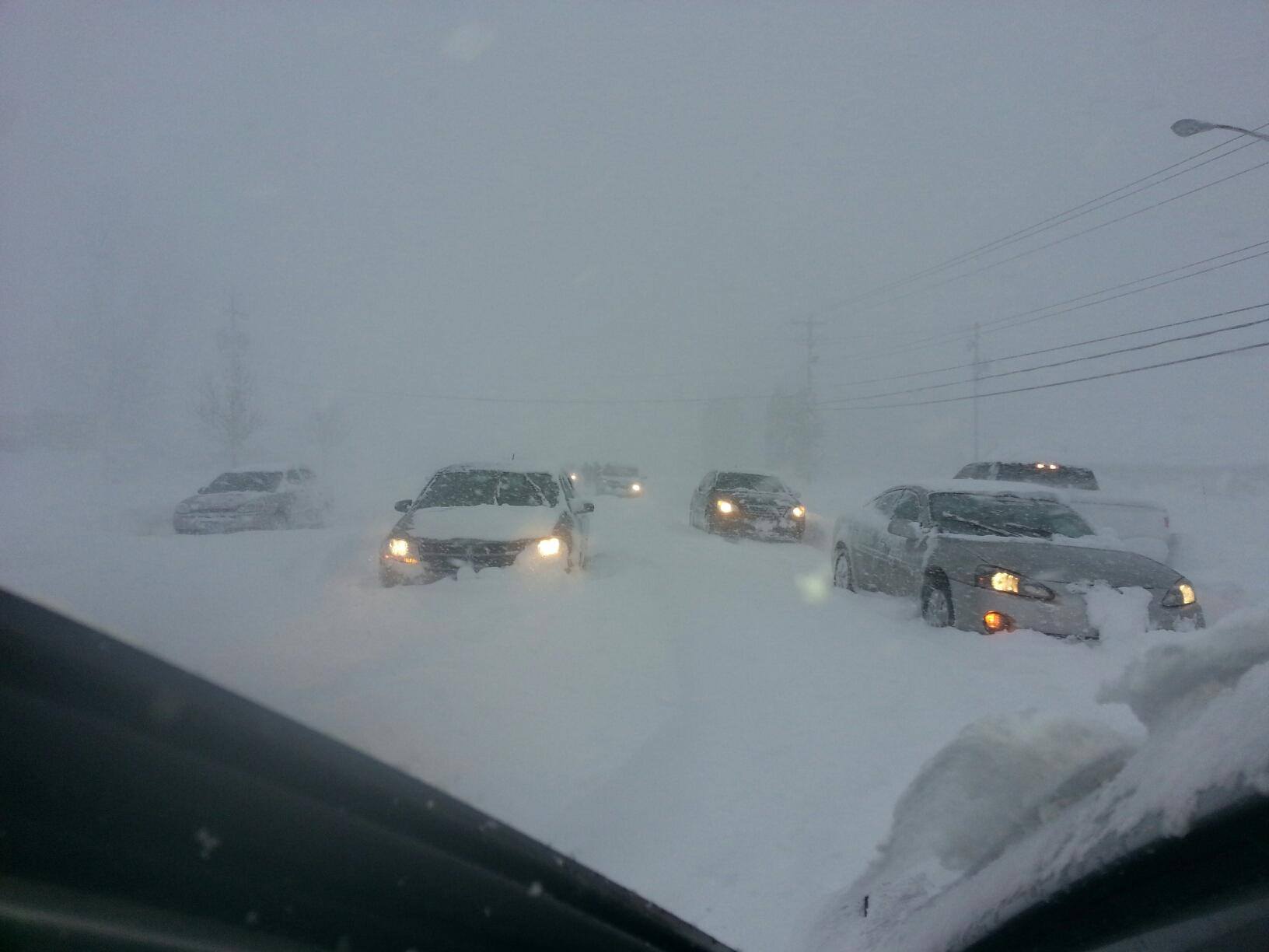
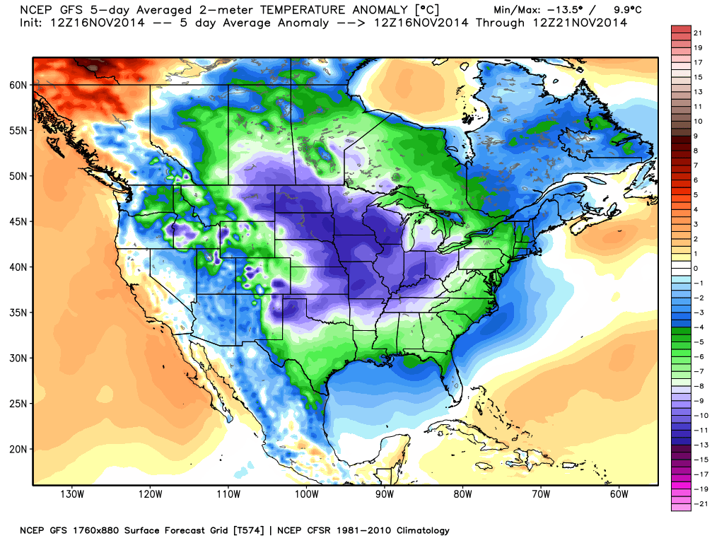
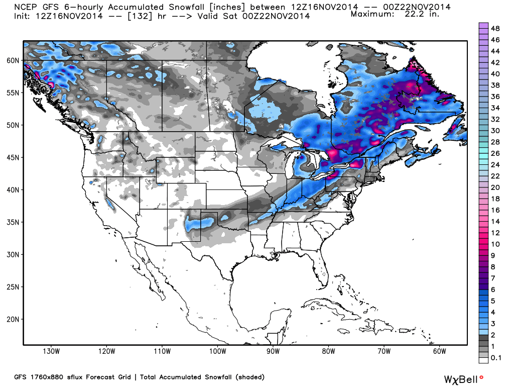
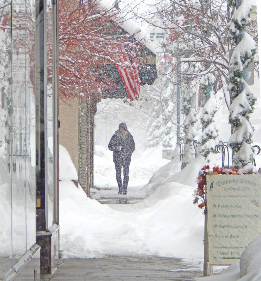
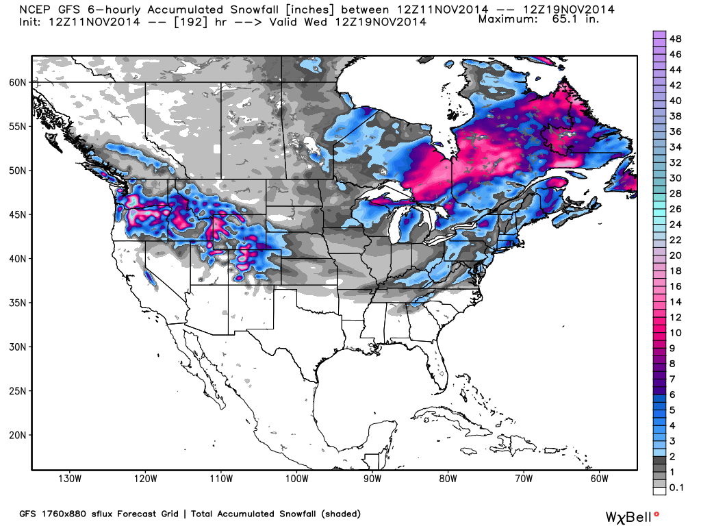
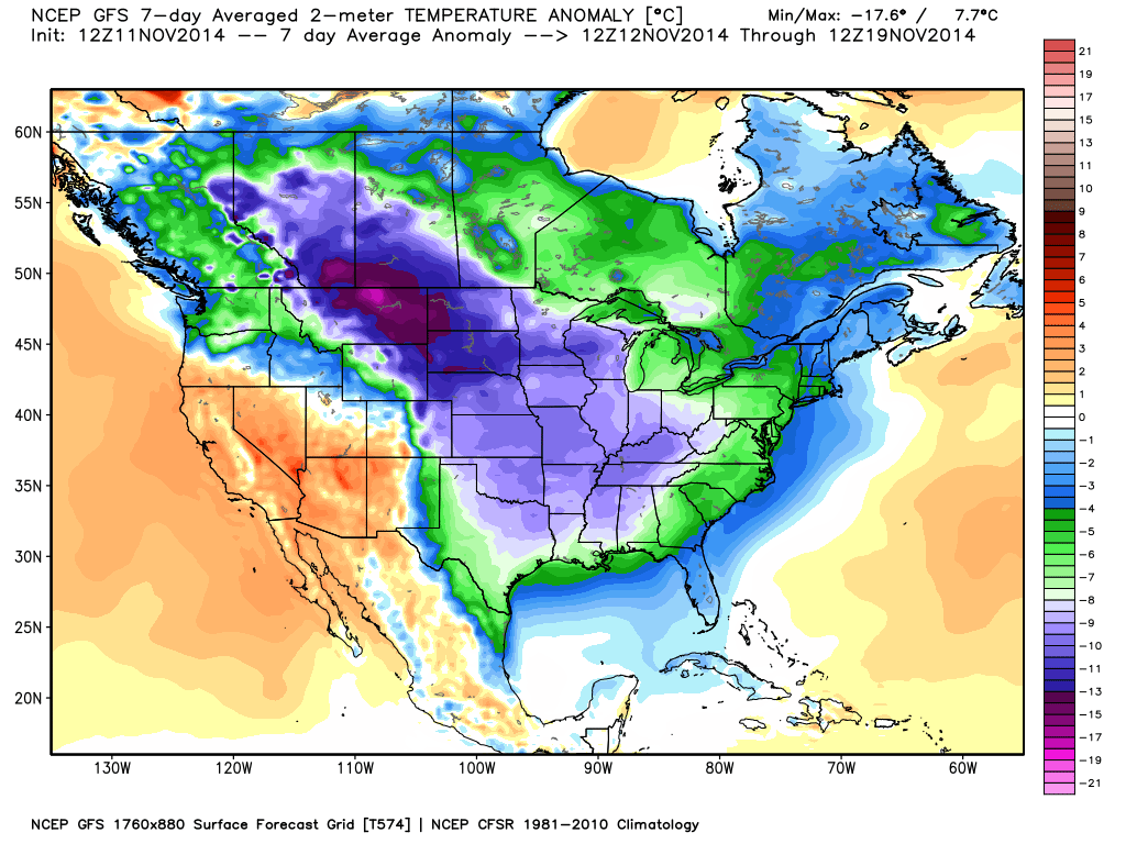
So, as the unseasonal cold settles in over the U.S. this week, don’t be fooled by those who claim “global warming causes cooling”. What we are seeing is natural variability, likely dominated by the oceans. The “new weather norm” might well be different from what anyone less than 30 years old has been used to.

To the extent that human-caused warming is occurring, I am increasingly convinced it is a largely benign — and possibly beneficial — needle lost in the haystack of Mother Nature’s natural climate gyrations.

With the spectacular cold event now spreading over much of the contiguous U.S. (and still expected to bring 30 below zero temperatures in Yellowstone Lake, WY tomorrow morning) the snow forecast for the next 8 days shows only 6 states that should miss snow (graphics courtesy of Weatherbell.com, click for full-size):

Those states are South Carolina, Florida, Louisiana, Mississippi, Texas, and Arizona. While it’s still very early, the 10-day forecast shows a potential major snowstorm for the mid-Atlantic and Northeast states late next week.

The 7-day average temperature departures from normal really are exceptional in their geographic extent, intensity, and persistence, with widespread 15-25 deg F below normal temperatures…averaged over 7 days:

Some locations in Montana, Wyoming and Colorado will have temperatures ranging 50 to 60 deg. F below their seasonal norms in the next couple of days.

It will be interesting to see if this month ends up being one of the coldest Novembers on record for the U.S.

Even though it’s still early November, a January-like cold wave just entering Montana and the Dakotas on Sunday will bring 30 below zero temperatures to scattered locations in Montana and Wyoming by Wednesday morning.

The cold will fill the nation’s midsection by mid-week, with no let up in sight. The coldest air to arrive in a series of reinforcing surges is still a week away.

Temperatures are forecast to run 15 to 30 deg. F below normal for at least 5 days over a large portion of the central U.S. starting late in the coming week (graphic courtesy of Weatherbell.com, click to enlarge):

On individual days the temperatures will be as much as 50 deg. F below normal for this time of year, which is quite exceptional. The air mass temperature (850 mb, ~5,000 ft. altitude) will be as much as 4.5 standard deviations below normal, which is less than 1 in 100,000 in probability terms.

Brace yourself for more “polar vortex” news stories by the middle of next week.

An unusually widespread and persistent cold air mass will grip all but the U.S. Southwest and Florida by late in the week.

It’s origins can be traced back to eastern Siberia a week ago, then it crossed the Arctic Ocean and northwest Canada. It will enter Montana and the Dakotas on Sunday, then gradually sink south and east as the week progresses.

The latest forecast for 7-day average temperature departures from normal shows widespread 10 to 15 deg. F below normal over much of the nation for the seven days starting next Wednesday (click for full-size, graphics courtesy of Weatherbell.com):

That’s a whole week of unusually cold weather, folks. Recent cold events have been very short-lived, sweeping through rapidly, lasting not much more than a day or so. This one is going to stick around.

The Arctic intrusion will be accompanied by a swath of snow across the Northern Plains and Great Lakes on Monday, then snow for Virginia and D.C. by Friday:

My friend Joe Bastardi at WeatherBell tells me the ocean temperature and weather patterns right now are reminiscent of the epic winters of 1976-77 and 77-78. I remember those winters. I was taking graduate meteorology courses at UW-Madison at that time, and the meteorology professors were all saying the early cold air outbreaks we experienced would surely end.

Except they didn’t.

The Version 5.6 global average lower tropospheric temperature (LT) anomaly for October, 2014 is +0.37 deg. C, up from the September value of +0.29 deg. C (click for full size version):

The global, hemispheric, and tropical LT anomalies from the 30-year (1981-2010) average for the last 22 months are:

YR MON GLOBAL NH SH TROPICS
2013 1 +0.497 +0.517 +0.478 +0.386
2013 2 +0.203 +0.372 +0.033 +0.195
2013 3 +0.200 +0.333 +0.067 +0.243
2013 4 +0.114 +0.128 +0.101 +0.165
2013 5 +0.082 +0.180 -0.015 +0.112
2013 6 +0.295 +0.335 +0.255 +0.220
2013 7 +0.173 +0.134 +0.211 +0.074
2013 8 +0.158 +0.111 +0.206 +0.009
2013 9 +0.365 +0.339 +0.390 +0.190
2013 10 +0.290 +0.331 +0.249 +0.031
2013 11 +0.193 +0.160 +0.226 +0.020
2013 12 +0.266 +0.272 +0.260 +0.057
2014 1 +0.291 +0.387 +0.194 -0.029
2014 2 +0.170 +0.320 +0.020 -0.103
2014 3 +0.170 +0.338 +0.002 -0.001
2014 4 +0.190 +0.358 +0.022 +0.092
2014 5 +0.326 +0.325 +0.328 +0.175
2014 6 +0.305 +0.315 +0.295 +0.510
2014 7 +0.304 +0.289 +0.319 +0.451
2014 8 +0.199 +0.244 +0.153 +0.061
2014 9 +0.294 +0.187 +0.401 +0.181
2014 10 +0.367 +0.335 +0.399 +0.191

It should be remembered that during ENSO, there is a 1-2 month lag between sea surface temperature change and tropospheric temperature changes, so the tropospheric temperature anomaly will take a month or two to reflect what recent global SSTs have been doing.

The global image for October should be available in the next day or so here.

Popular monthly data files (these might take a few days to update):

uahncdc_lt_5.6.txt (Lower Troposphere)
uahncdc_mt_5.6.txt (Mid-Troposphere)
uahncdc_ls_5.6.txt (Lower Stratosphere)

When a tropical cyclone moves poleward and merges with a frontal system, and then draws upon the extra energy that exists between cold and warm air masses, a Sandy-type storm can result.

Sometimes it causes explosive cyclogenesis, what we call a “bomb”, with rapidly deepening low surface pressures.

I’ve been watching Super Typhoon Nuri in the West Pacific, one of the strongest of the year, and each run of the GFS model continues to show this system becoming a spectacular extratropical storm in the Bering Sea, with hurricane force winds and near record low barometric pressure in about 5 days time, after it just misses Japan.

As of today, this is what Nuri looks like in the latest MODIS imagery…it’s not a particularly large storm, but it has an intense core, with maximum surface winds estimated at 180 mph with gusts to 220 mph (these are satellite-estimated…they do not routinely fly into typhoons to measure them like we do in the West Atlantic):

Here’s some nice video of Nuri from the International Space Station from yesterday:

The GFS forecast model run from this morning shows Nuri as an extratropical low with an exceedingly low central pressure of 924 mb (27.29 inches) by Friday evening (graphic courtesy of Weatherbell.com, click image for full-size):

The previous 2 model runs had the low at 919 mb lowest pressure. By comparison, the lowest pressures recorded in extratropical storms have been in the range of 912-920 mb, in the North Atlantic, so it looks like Nuri might be one of the strongest on record. The lowest surface pressure ever recorded in the U.S. was from one of these Bering Sea systems: 927 mb (27.35 inches) at Dutch Harbor, Alaska on October 25, 1977.

As I predicted two days ago, the earliest snows on record are beginning to occur in the Carolinas.

Columbia, SC has just experienced their earliest snow in 125 years of weather records, beating the Nov. 9, 1913 earliest snow record by 8 days. Current South Carolina weather shows it’s still snowing in Greenville, SC.

The Christian Science Monitor is reporting Greenville was especially hard hit with downed trees and power outages. The Smokey Mtns received up to 16 inches overnight. The current U.S. snow cover map shows 18 states with some amount of snow this morning.

Here is the latest model forecast of total snowfall ending at midnight tonight (graphic courtesy of Weatherbell.com):

Early indications are that next Sunday the “polar express” will arrive in the northern plains and Great Lakes with bitterly cold air currently sitting over northern Siberia.

The validity of the satellite record of global temperature is sometimes questioned; especially since it shows only about 50% of the warming trend as do surface thermometers over the 36+ year period of satellite record.

The satellite measurements are based upon thermal microwave emissions by oxygen in the atmosphere. But like any remote sensing technique, the measurements include small contaminating effects, in this case cloud water, precipitation systems, and variations in surface emissivity.

A new paper by Weng et al. has been published in Climate Dynamics, entitled “Uncertainty of AMSU-A derived temperature trends in relationship with clouds and precipitation over ocean”, which examines the influence of clouds on the satellite measurements.

To see how clouds and precipitation can affect the satellite temperatures, here’s an example of one day (August 6, 1998) of AMSU ch. 5 data (which is used in both our mid-tropospheric and lower-tropospheric temperature products), and the corresponding SSM/I-derived cloud water for the same day:

As can be seen, the contamination of AMSU5 by cloud and precipitation systems is small, with slight cooling in deep convective areas, and no obvious cloud water contamination elsewhere (cirrus clouds are essentially transparent at this microwave frequency).

And even if there is contamination, what matters for tropospheric temperature trends isn’t the average level of contamination, but whether there are trends in that contamination. Below I will discuss new estimates of both the average contamination, as well as the effect on tropospheric temperature trends.

The fact that our monthly gridpoint radiosonde validation shows an extremely high level of agreement with the satellite further supports our assumption that such contamination is small. Nevertheless, it is probably worth revisiting the cloud-contamination issue, since the satellite temperature trends are significantly lower than the surface temperature trends, and any potential source of error is worth investigating.

What Weng et al. add to the discussion is the potential for spurious warming effects in AMSU ch. 5 of cloud water not associated with heavy precipitation, something which we did not address 18 years ago. While these warming influences are much weaker than the cooling effects of precipitation systems (as can be seen in the above imagery), cloud water is much more widespread, and so its influence on global averages might not be negligible.

The Weng et al Results Versus Ours (UAH)

I’m going to go ahead and give the final result up front for those who don’t want to wade through the details.

Weng et al. restrict their analysis to 13 years (1998-2010) of data from one satellite, NOAA-15, and find a spurious cooling effect from cloud contamination in the middle latitudes, with little effect in the tropics. (They don’t state how they assume their result based upon 13 years, even if it was correct, can be applied to 35+ years of satellite data.) I’ve digitized the data in their Fig. 8, so that I can compare to our results (click image for full size):

There are two main points to take away from this figure. First, the temperature trends they get at different latitudes for 1998-2010 are VERY different from what we get, even in the “all-weather” case, which is simply including all ocean data whether cloud-contaminated or not. The large warming signal we get in the tropics is fully expected for this limited period, which starts during a very cool La Nina event, and ends during a very warm El Nino event.

I have spent most of this week slicing and dicing the data different ways, and I simply do not see how they could have gotten the near-zero trends they did in the tropics and subtropics. I suspect some sort of data processing error.

The second point (which was the main point of their paper) is the difference in “clear-sky” versus “all-weather” trends they got in the middle latitudes, which is almost non-existent in our (UAH) results. While they estimate up to a 30% spurious cooling of warming trends from cloud contamination, we estimate a global ocean average spurious cooling of only -0.006 deg. C/decade for 1998-2010 from not adjusting for cloud-contaminated data in our operational product. Most of this signal is probably related to the large change in cloud conditions going from La Nina to El Nino, and so it would likely be even less for the 36+ year satellite record.

While I used a different method for identifying and removing cloud contamination (I use localized warm spots in AMSU ch. 3, they use a retrieval scheme using AMSU ch. 1 & 2), I get about the same number of data screened out (40%) as they do (20%-50%), and the geographic distribution of my identified cloud and precip. systems match known regional distributions. So I don’t see how different cloud identification methodologies can explain the differences. I used AMSU prints 10-21 (like our operation processing), as well as their restricted use of just prints 15 & 16, and got nearly the same results, so that can’t explain the discrepancy, either.

I have many more plots I’m not showing relating to how cloud systems in general: (1) do indeed cause a small average warming of the AMSU5 measurements (by up to 0.1 deg. C); (2) less frequent precipitation systems cause localized cooling of about 1 deg. C; (3) how these effects average out to much smaller influences when averaged with non-contaminated data; and most importantly (4) the trends in these effects are near zero anyway, which is what matters for climate monitoring.

We are considering adding an adjustment for cloud contaminated data to a later version of the satellite data. I’ve found that a simple data replacement scheme can eliminate an average of 50% of the trend contamination (you shouldn’t simply throw away all cloud-influenced data…we don’t do that for thermometer data, and it could cause serious sampling problems); the question we are struggling with is whether the small level of contamination is even worth adjusting for.